YMEC software
| TOP
| STORE
| DSSF3
| RAE
| RAD
| RAL
| MMLIB
| FAQ
| Support
| Contact Us
|

This site provides information for how to perform the
sound measurement and analysis by using standard Windows PC. Realtime Analyzer, Sound
Analyzer, and Environmental noise Analyzer turn your PC into a
measurement laboratory. Covered field is audio measurement and adjustment, room
acoustics, electronic measurement, acoustic analysis of noise, human voice, musical instrument, and
medical auscultation sound. You can do the same measurement by your own notebook
PC. Go to YmecStore
to download the sound measurement and analysis software DSSF3.
| Japanese | English |
Introduction to the autocorrelation function (ACF)
In the sound measurement and analysis software, DSSF3,
sound is analyzed by use of the ACF in addition to the conventional FFT
analysis. We provide some information about the ACF in this page.1. Introduction
Sound is a variation of the air pressure transmitted from a sound source.
The pressure variation can be expressed as a waveform. Sound is transmitted
with progress of time. If time does not exist, we cannot hear sound. Please keep in mind that the
ACF is a useful tool by which we can investigate
sound in the time domain.
2. Time domain and frequency domain of sound
There are two methods of describing sound. One is the method in the time
domain ("waveform" or "ACF", as functions of time). The
other is the method in the frequency domain ("spectrum" as a function
of frequency). These two methods describe a same sound from different points of
view, and
the conversion from each other is possible. That is, although sound can be
similarly described effectively whichever we use, one of methods is more convenient
than another in some situation. For example, you often see the bar graph
(graphic equalizer) in a component stereo. It shows the frequency distribution
of sound. You can grasp easily that how much amount of low-pitched sound
or high-pitched sound is contained. In contrast, the ACF analysis that we offer
is effective in order to focus on the temporal information of sound such as
periodicity or sudden transition.
3. The relation between sound and our brain
The sound coming into the ear progresses along a hearing pathway, and is
perceived with the passage of time. At this time, the meaning of the sound is
interpreted by our brain at every moment. Here is the importance of analyzing
sound in time domain. Except that the ACF describes the sound in time domain,
the same mathematical information is expressed in the power spectrum. However,
the ACF analysis differs from the spectrum analysis greatly in that the
higher-level processes in our auditory brain are taken into consideration. If
you are interested in the neural mechanism of analyzing sound by use of the ACF,
visit cariani.com to see
the latest research topics.
4. What is autocorrelation function?
Autocorrelation function (ACF) is defined by the following formula.
-
- - - - -(1)
Here, p(t) is the sound waveform, t is the delay time and 2T
is the integration interval. As explained previously, the analyses in the time
domain and the frequency domain are mutually convertible. When the power
spectrum of a sound signal is defined as Pd
(w), the ACF (F(t)) is
obtained as follows.
-
- - - - -(2)
-
- - - - -(3)
Thus, ACF and the power spectrum include the same information mathematically.
Now, let us consider the physical meaning of the ACF.

Fig.1 The physical meaning of the autocorrelation function and the sound
signal at t= 0 and t=t1
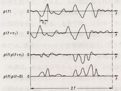
As shown in Fig. 1, let's consider the signal p(t) and its delayed version p(t+t).
If the amplitude of p (t) and p (t+t)
is large, and two signals are similar, the correlation value of two signals,
Fp(t)
becomes large. So, it can be said that the ACF is the function that shows
how much similarity is included in the signal itself. The ACF is a useful tool
in the signal analysis because it can be used to detect the periodicity of the
signal. Below, the examples of the ACF for
music and noise are shown.
| Music |
|

Time [ms]
|
| Noise |
|

Time [ms]
|
We can see that the ACF of the noise signal becomes small immediately. This
means that the similarities between the original signal and the time delayed
signal are low, because
various sound components are contained in noise. In contrast, the ACF of the
music has several periodicities and decreases gradually. The maximum peak found
at 20 ms corresponds to the fundamental frequency of the signal. We can see that
the ACF is repeated with this fundamental period (peaks are found at 40 ms, 60
ms, and 80 ms). In most cases, the fundamental frequency is perceived as pitch.
Other peaks within the fundamental period corresponds to the strong
harmonics.
5. Significant parameters from the ACF
Any sound signals (e.g. music, environmental noise, speech,
singing voice) can be analyzed using the
following four factors extracted from the ACF.
(1) Average sound energy: F(0)
It expresses the power of sound. There is a close relationship between F(0)
and the subjective scale of loudness.
(2) Effective duration of the ACF: te
This is defined as the delay time where the envelope of the normalized ACF decays to
0.1. The reverberation component contained in the
signal itself is expressed. For example, slow orchestra music has much longer te
than speech. Here, the normalized ACF is defined by the following formula.
-
- - - - -(4)
The figure below shows the definition of te.
The ACF plotted in the logarithmic scale can be fitted by the linear regression
in most cases.
(3) Time delay of the maximum peak: t1
This corresponds to the pitch of sound.
(4) Amplitude of the maximum peak: f1
This corresponds to the pitch strength of sound.
6. Application of the ACF
As shown above, the factors extracted from the ACF have close relation with the
subjective attributes of sound. In the field of architectural
acoustics, the most preferred delay time of the reflective sound and the
reverberation time can be calculated by using the effective duration of the
music signal's ACF. By
this approach, design of the excellent concert hall has been attained. Basic
research using the ACF analysis can be found at http://www.andolab.org/
| TOP | STORE
| DSSF3
| RAE | RAD
| RAL | MMLIB
| FAQ
| Support | Contact Us |
If you have questions or comments about this page,
feel free to contact us by email ymec@ymec.com or by online
inquiry form.