| Japanese | English |
This time, I report the running ACF analysis of the idling sound of Ferrari Mondial by changing the analysis condition. Time resolution of the analysis is set to finer than before.
It is said that human brain is catching music by the time window of 2 - 3
seconds. It is the reason that I have performed the analysis with the
integration time of 2 seconds (car2.htm). The integration time is now set to 0.2 seconds to analyze the same
sound in more detail.
![]() ferrari1.wav (44.1kHz / Stereo / 15sec / 2,585KB)
ferrari1.wav (44.1kHz / Stereo / 15sec / 2,585KB)
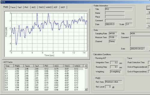
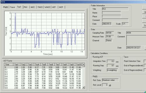
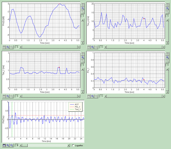
F(0): This graph shows a time course of the sound level measured by the higher time resolution than before. It can be seen that detailed change of the sound level is measured now. Listening the sound carefully, the impression of the variation in sound may be closer to this graph.
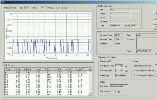
Next, let's see the graph of tIACC. This parameter measures the time delay of two channel signals. It expresses the arrival direction of sound received by the stereo microphones. A negative value of the tIACC shows that the sound is coming from the right side of microphones. In contrast, when the sound source is located on the left side of the microphones, it becomes positive.
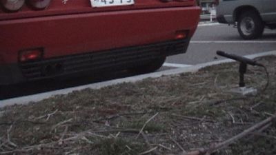
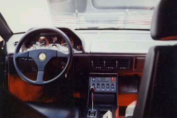
The main sound sources in this case are mufflers on both sides. See the above photo. So, the fluctuation in tIACC implies that two sounds become louder and weaker repeatedly in every moment. The point of the minimum sound level at 0.9 seconds (see the above graph) seems to be the alternating point of the sound sources. Even though the microphones have not been set correctly to a sound source, the relative positions of two or more sound sources can be shown correctly.
t1 (Pitch ): Dominant frequencies of sounds from silencers on both sides and the engine are shown. When the integration time was 2 s, the dominant frequency was always 360 Hz (i.e. t1 was always around 2.7 ms). But this time, it can be seen that the engine noise sometimes has the dominant frequency component around 1 kHz and 2 kHz (say, t1 is 1 ms and 0.5 ms). When the exhaust noise is louder, the dominant frequency becomes 360 Hz.
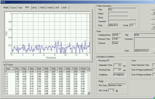
f1 : Pitch strength is also fluctuating.
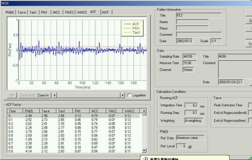
This is the ACF waveform measured at 0.9 s.
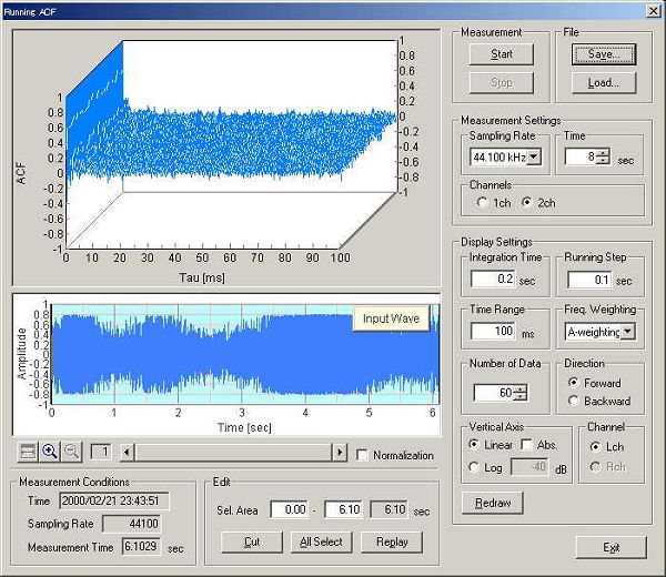
Next, the result of other engine noise is shown. This sound was measured on February 21 2000. It was measured just above the engine with the engine hood open.
![]() ferrari5.wav (44.1kHz / Stereo / 6.1sec / 526KB)
ferrari5.wav (44.1kHz / Stereo / 6.1sec / 526KB)
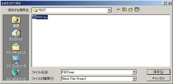
Sound was saved as .wav format.
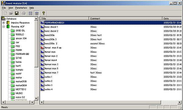
Data is load by SA.
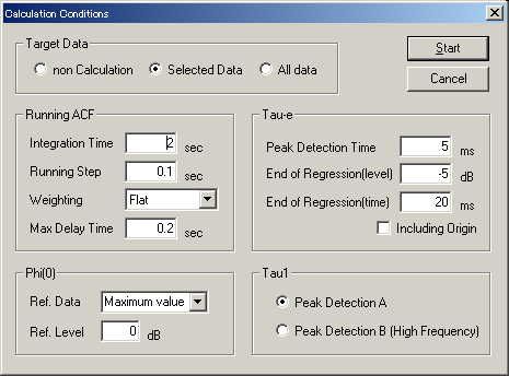
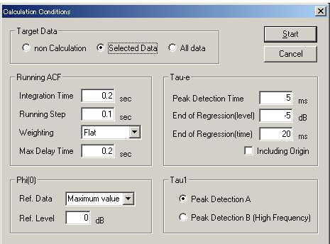
The calculation condition. Integration time was first set to 2 s.
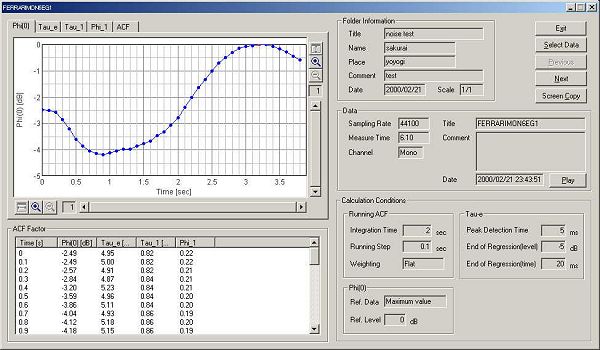
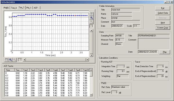
This is a time course of the sound level.
τ1 values.
Now the same sound was analyzed with 0.2 s integration time.
Analysis result.
τ1 values
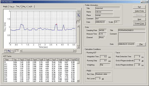
When the sound is analyzed with the short integration time, time change of the analyzed values becomes fine. While the dominant frequency component is same in most time, it changes sometimes.
DSSF3 is a multi-dimensional sound analysis software. Much information are collected, such as the time course of the sound level, pitch, pitch strength, and so. By using those information, adjustment and diagnosis of the engine may become possible.
April 2003 by Masatsugu Sakurai