| Japanese | English |
In this series of measurement report, sound wav files will be analyzed by the autocorrelation function. Sound source is a piece of anechoic recordings of a piano music. Other sound files can be downloaded from "Sound preference audition room".
In a concert hall, reverberation of a room is added to the sound of the musical instruments. In contrast, there is a special environment in which there is no reverberation. It is called an anechoic room. In the anechoic room, we hear only a sound which the musical instrument itself emits. By the reverberation, what effect is added to the sound? This is a primary question of this analysis.
At first, one of the analysis conditions "suitable analysis time (temporal window length)" is checked from the 3D display of the running autocorrelation.
| Date: | 20 Sep. 2002 |
| Place: | Apartment |
| Personal computer: | DELL INSPIRON 5000e |
| OS: | Windows 2000 Professional |
| Software: | DSSF3 |
| Piano dry source: |
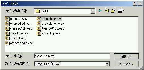
First, download this file. Right-click on the piano1sc.wav above, and select "Save Target As...". "Save As" dialog will appear, where make a new folder and save the file in it.
DSSF3 can load the wave file. In the "ACF measurement" screen, click on the "Load..." button and select the file. If you are not using DSSF3, you need to play the wave file by the Windows Media Player and to get the RA to load it. (A input device of RA is set to "wave" or "mixer".)
In the running ACF display of RA, click the "Load" button.
Select the downloaded wav. file.
Top figure is the running ACF of the loaded file. The bottom graph is a temporal waveform of the sound.
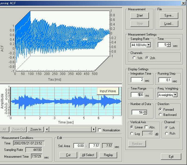
This is the running ACF analysis of a piano music. The integration time and the running step are 2.0 and 0.1 seconds. Displayed time range is 0.5 second. It is said that the integration time of 2.0 second is the suitable temporal window for the general music motif (Architectural acoustics, by Yoichi Ando).
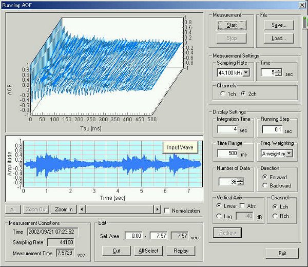
The same music was recalculated with the integration time of 5.0 second. The ACF display is almost flat, because the signal is averaged in a long duration. It seems that the information of the music signal cannot be expressed with this setting.
Though a 3D display of the ACF is a good way for displaying a music signal smoothly, it is difficult to see the temporal fluctuation of sound in detail. It is necessary to further analyze sound by the Sound Analyzer. Below, an example of the analysis results by the Sound Analyzer is shown.
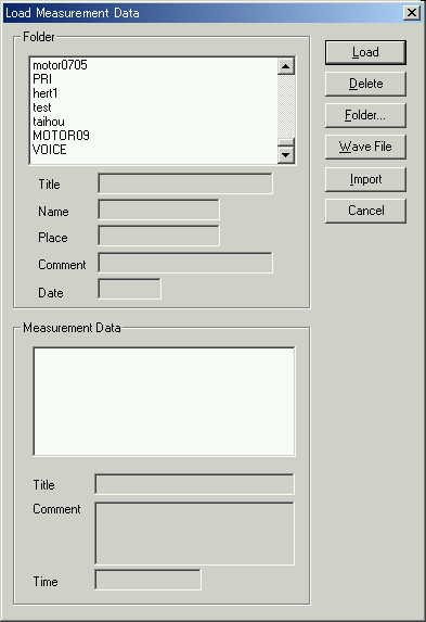
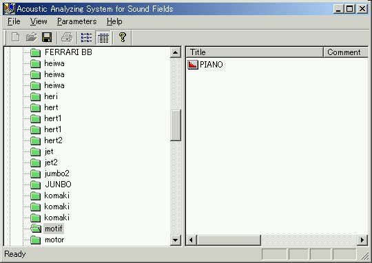
To analyze data, save the loaded sound on the Realtime Analyzer's Running ACF window. Click the Save button on the top of the window, and follow the instruction. Once you save data, open Sound Analyzer. Below is the main window of Sound Analyzer. Saved data will be displayed. To analyze data, select a data folder and click Parameters > Calculation, from the menu bar.
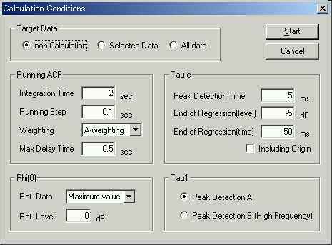
This is the calculation conditions window. Set the values as below.
Analysis results. Top left graph is a time history of the sound intensity. Other graphs represent important acoustic parameters, but it is not explained here. By comparing the sound intensity graph with the temporal waveform of the sound (see above), time resolution of this analysis is very rough. It may be possible that shorter integration time would be necessary to analyze sound more appropriately.
September 2002 by Masatsugu Sakurai