| Japanese | English |
At that time, I found that the aircraft noise consists of at least two prominent components. One is the fan exhaust noise and the other is the exhaust from the jet engine. The fan exhaust noise emits the very high frequency component, and the jet engine exhaust emits the low frequency noise.
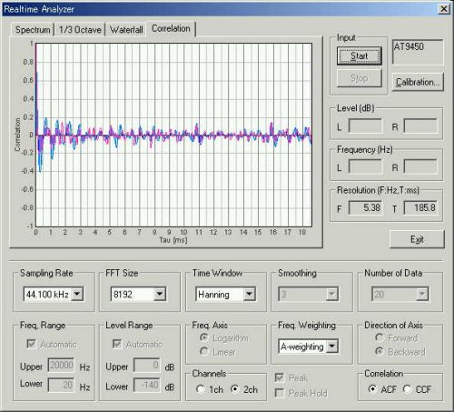
However, at the first measurement, DSSF3 did not have the high time resolution FFT analyzer that works with the ACF analysis. So, I estimated those frequencies by using the real time spectrum analyzer and the running ACF graphs separately. However, it took much time, and the time constant for the measurement might not be suitable for the analysis of such noise. Since the FFT was performed on an arbitrary portion, it was lacking in reproducibility. These limitations did not allow me to investigate the quality of noise appropriately. To overcome these limitations, DSSF3 has been improved as follows.
DSSF3 News 1
Jul 2003
Display of the Running ACF results [SA]
In the graph of analysis results, red mark is displayed on the specified point.
Now, it has been improved so that it is easy to treat a numerical data table.
Signal waveform and spectrum display are added [SA]
Temporal waveform and spectrum were added to the graph display of the ACF
analysis.
In the current version of DSSF3, the FFT analysis and the ACF analysis can be performed on exactly the same data. So, I decided to analyze the same data again. The results of the new analysis are reported in this page after the original report.
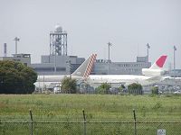
We went to Nagoya Airport to conduct a preliminary
analysis of passenger jet noise.
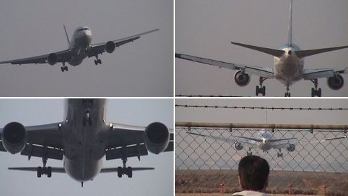
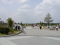
The measurements were taken adjacent to the landing lights
along the runway for incoming jet passenger planes at the airport. (= position 1
shown in the following map)
 |
  |
PASSENGER JET LANDING
The autocorrelation function (ACF) is almost constant during the
measurement.
The running ACF was measured from the recorded sound. To perform the same analysis described in this page, download the wav file below and load it on the Running ACF window.
![]() air1.wav (44.1kHz / Stereo / 15sec / 2.52MB)
air1.wav (44.1kHz / Stereo / 15sec / 2.52MB)
Now let us take a look at the effective duration of ACF, te. See Introduction of the autocorrelation function for detailed explanation of the acoustic parameters calculated from the ACF. The next graph shows the te values for the same 13-second period as above. The te during the approach remains constant at about 5 ms.
As the aircraft approaches, t1 is constant at about 0.5ms. In other words, the fundamental frequency of the engine sound is 2 kHz, because t1 is the reciprocal of the fundamental frequency (1000 ms / 0.5 ms = 2000 Hz).
Pitch strength (f1) is about 0.1. Engine sound is a noise-like sound that does not have tonal component.
Next is the 1/3 octave analysis. This is used in the usual noise measurement. As is
shown, we think that the ACF analysis gives more information than the sound level meter.
January 2002 by M. Sakurai
From here, written in 2004/07/16
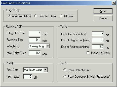
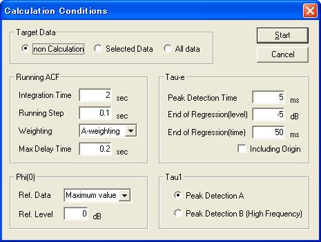
The same data air1.wav was analyzed in SA. The calculation conditions are shown in the figure below. The integration time of 2 sec and the running step of 0.1 sec is chosen. It means that the 2.0 s portion of data portion is analyzed in every 0.1 s.
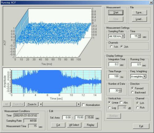
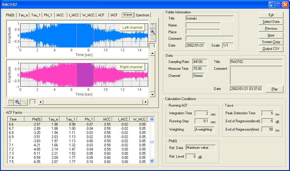
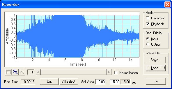
The next figure is the analysis result window. In the new version of SA, graph displays of Wave and Spectrum are added. This is the temporal waveform of the aircraft noise. The blue area indicated in the waveform display corresponds to the analyzed data portion listed in the ACF factor table. In this example, the area between 6.6 and 8.6 s is selected. The duration of 2.0 s is decided by the "Integration time".
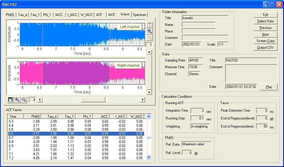
The next figure is the waveform display too, but now it is zoomed in to x8. This resolution has also been improved in the current version of SA. The measured sound can be listened to by clicking the "Play" button in this window. Analysis results can be saved as a text data.
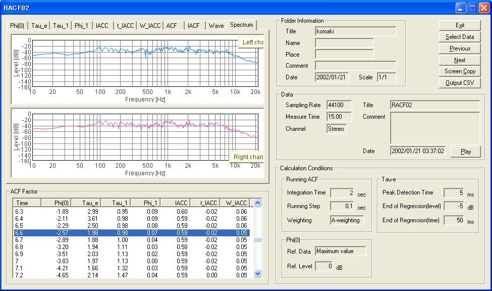
Next, I proceed to the spectrum display. Power spectrum can also be seen on the selected data portion indicated by the blue area.
The figure below shows the spectrum of data between 6.6 and 8.6 s. It is very convenient that the analysis results of the same data portion are displayed by changing the graph display tab. The ACF and the spectrum are easily compared.
From this spectrum, I can see that the prominent frequency of this jet noise is at about 1.1 kHz. Higher harmonics are found at 2.2, 3.3, 4.4, and 5.5 kHz.
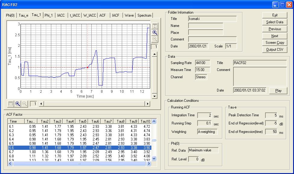
The next figure shows the time course of the ACF parameter, τ1. The τ1 value is the first peak in the ACF, and its reciprocal corresponds to the prominent frequency. At 6.6 s, τ1is 0.98 ms, corresponding the 1000 / 0.98 = 1020 Hz. I can see that the τ1 is increasing (meaning that the prominent frequency is decreasing) until 7.5 s. Then it abruptly decreases.
The graph is zoomed in to this portion, between 7.7 and 8.1 s.
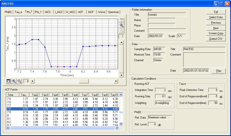
At 7.8 s, τ1 is 0.16 ms, so the prominent frequency is 1000 / 0.16 = 6250 Hz.
It was found that the prominent frequency of jet noise is about 2 kHz when the aircraft is approaching. This may be due to the fan exhaust noise. I assume that this frequency depends on the the engine power, the speed, and the type of the aircraft.
Next, the same sound was analyzed by the spectrogram. To analyze sound, the wav file (air1.wav) was loaded on the recorder.
Open the spectrogram, set the Time Range to 15 s (to match the length of sound file), and set the Direction of Axis to Fwd. By clicking the Start button on the window, sound file will be replayed and its spectrogram will be drawn. The spectrogram clearly displays the temporal variation of the spectrum.
In the figure below, it can be seen that the energy of the aircraft noise ranges from 100 Hz to 15 kHz throughout the recording. Strong energy components between 1 kHz and 5 kHz appear at around 4 seconds. As the frequencies of strong harmonics (i.e. red curves) are decreasing from 5 s to 8 s, we know that the airplane is reaching. Two components at 1.5 kHz and 2.5 kHz may correspond to the formants (F1 and F2) as it is compared to the human voice.
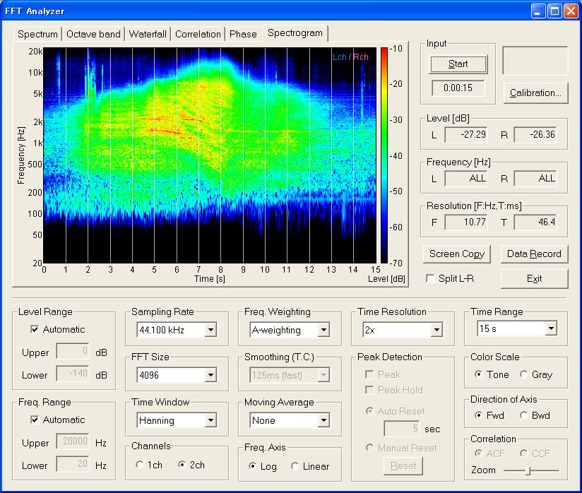
Spectrogram view can visualize very clearly what happens to the sound as the airplane is landing.
2005/07 Updated, Masatsugu Sakurai