| Japanese | English |
New analysis results by the latest version of DSSF3 is added to the original report written in January 2002.
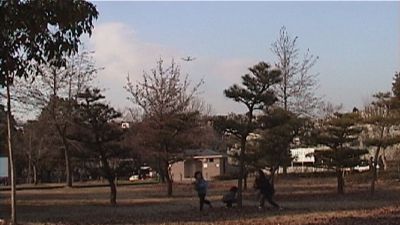
Airplanes approaching Nagoya Airport fly over residential areas. This
measurement was conducted at the Heiwa Park in Nagoya. The park is located just
west of the Nagoya exit from the Tomei Expressway. Jet engine noise is a
nuisance to local inhabitants, so flight paths are routed over mountainous and
other sparsely inhabited areas to the extent possible.
Nagoya Heiwa Park is essentially a large cemetery that was laid out after the
war in a hilly section in the eastern part of the city. Nagoya Airport is about
20 kilometers away from the park, so approaching aircraft are flying fairly low
when they pass over the park. Traveling at a speeds of about 500 kilometers per
hour, it takes a plane about 2 minutes and 30 seconds to cover 20 km, so the
planes are approximately 2 to 3 minutes away from touching down at the airport.
In recent years there has been substantial expansion of residential areas, so
complaints about environmental noise pollution have multiplied from people who
now in flight paths approaching the airport.
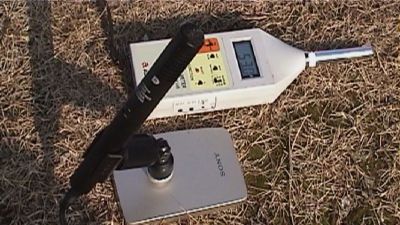 |
Microphone and a sound-level meter. Meter reading is 57 dB. Since the measurement site is a public park and vehicles come close, there is a certain amount of background noise. But it is much lower than the jet noise. |
 |
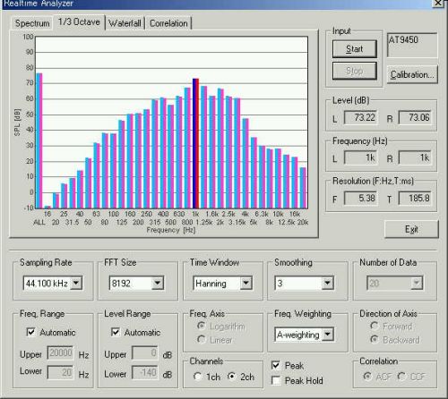
SONY VAIO laptop computer used for the measurement. It is difficult to see the display because of the sunlight on the LCD screen, but the software is working for checking the ordinary background noise using the 1/3 octave analysis. |
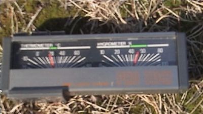 |
Temperature and humidity reading are 19 degree Celsius and 48 %, respectively. |
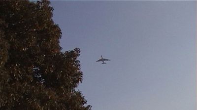 |
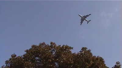
A jet is approaching overhead. I wanted to get the trees in the picture so I waited for this moment. |
 |
Now the plane is directly overhead. |
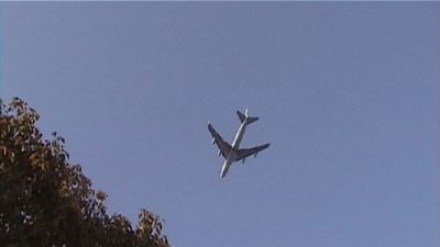 |
And now it is passing over. |
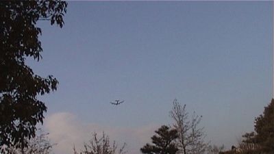 |
The plane is now pretty far from our measurement site. |
 |
The plane is flying just over the park. |
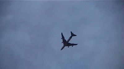 |
Here is a plane that we measured. |
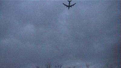 |
And one more shot. |
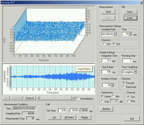
The next figure shows the running ACF measurement. It is a real-time measurement, so the integration interval was set to short (0.2 seconds). This setting reduces the calculation cost. For the analysis in detail, the data is recalculated by SA (Sound Analyzer) later.
![]() air2.wav (44.1kHz / Stereo / 30sec / 5.04MB)
air2.wav (44.1kHz / Stereo / 30sec / 5.04MB)
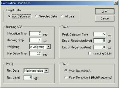
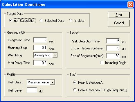
This is the calculation conditions for the analysis by SA.
F(0): Relative sound pressure level. From this figure we can see that the dynamic
range of the sound level is about 20 dB.
Next, the te is about 5 ms. This is the same level
as the Nagoya Airport measurement.
The next figure is the time course of t1,
reciprocal of the fundamental frequency. Could this be attributed to the Doppler effect? The frequency
is increasing as the airplane is approaching. In the Nagoya Airport measurements, roughly the
same waveform was recorded.
The pitch strength, f1, increases
during the plane is approaching. 
This is an example of the ACF measured at 8.2 sec after the measurement
starts. In this ACF, the first peak is at 0.6 ms (though it is below 0) and the largest peak is at 1.9
ms. Those peaks correspond to 1.5 kHz and 600 Hz respectively.
January 2002 by Masatsugu Sakurai
From here, written in 2004/08/08
This time, the same data is reanalyzed by the latest function of DSSF3. The waveform, the spectrum, and the ACF are compared. Before describing the results, I explain how to perform the measurement. You can obtain exactly the same result as in this report by following the procedure described below.
First, download the sound file air2.wav (44.1kHz / Stereo / 30sec / 5.04MB) on your hard disk. Right click the file name to download it.
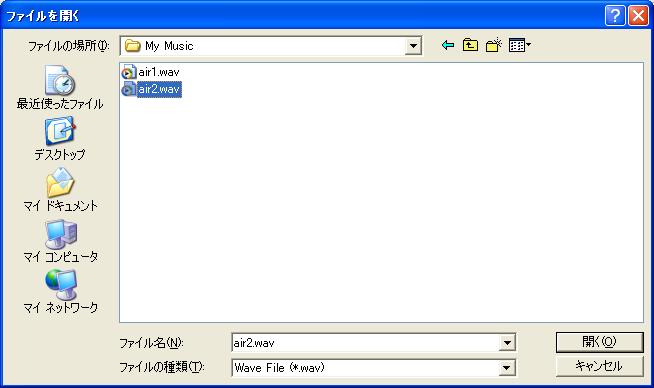
Then, load the downloaded sound file in RA. Start RA, open the "Running ACF" window, and click the "Load" button. The "Load Measurement Data" dialog appears. Click the "Wave File" button and open the file "air2.wav".
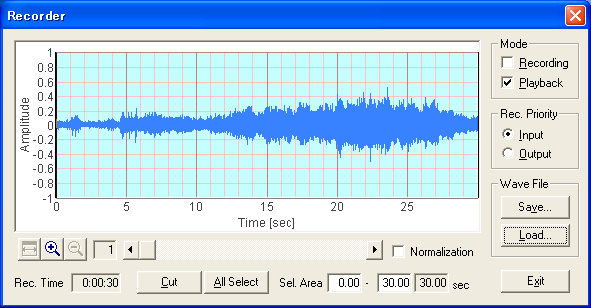
After loading the sound file, the measurement result immediately appears as shown in the figure below. The above graph shows the 3D display of the running ACF. The bottom graph is the waveform of the input data. By changing the display settings, the appearance of the running ACF display changes. But note that the detailed analysis is performed in SA (Sound Analyzer).
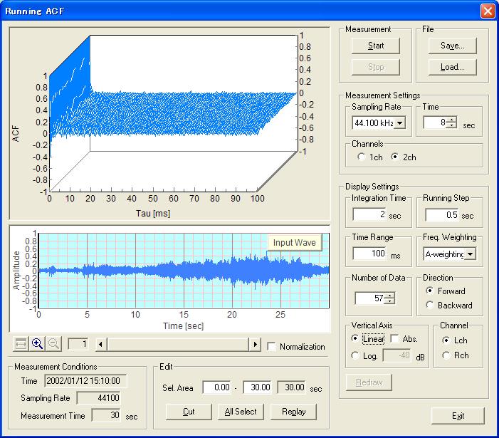
You can listen to the loaded sound by clicking the "Replay" button in the bottom of the Running ACF window. Replay time is indicated by a green line on the waveform display.
When you listen to air2.wav, you can notice that a voice of children is recorded at the beginning. This is an unwanted sound for noise measurement. If you like, this data portion can be cut. Right click and drag the mouse on the graph to select the portion, then click the "Cut" button. Only the selected portion will remain.
In the following, I analyze all of data because the level of the children's voice seems quite small in comparison with the aircraft noise in this case.
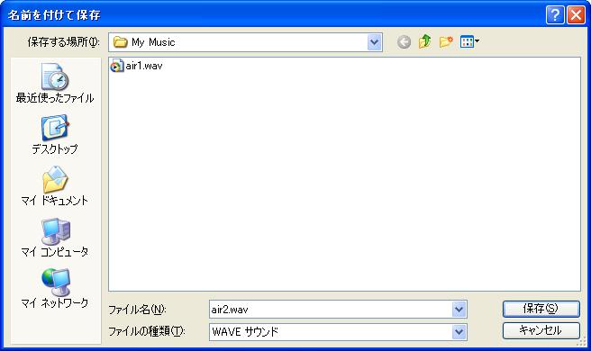
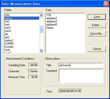
To start the analysis in SA, you have to save the data on the Running ACF window. Click the "Save" button to save the data. The "Save Measurement Data" dialog appears as below. In this example, I saved the data as "air2wave".
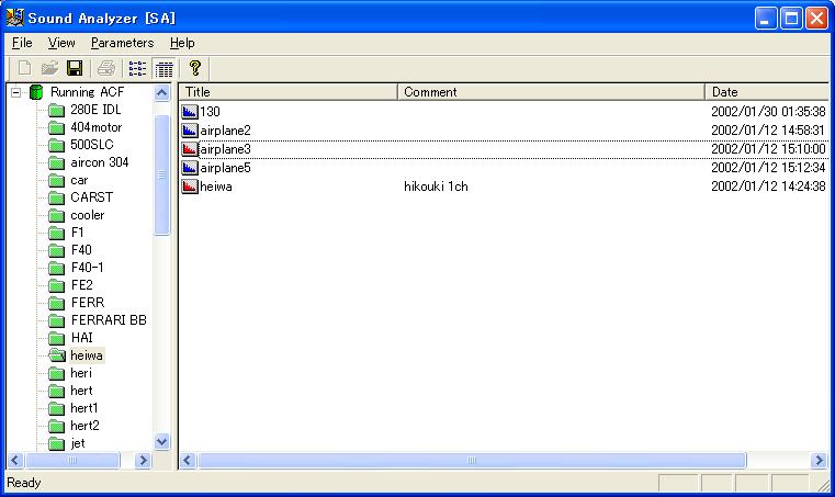
Then, start SA. Saved data appears in the data folder.
To start the analysis, select Parameters > Calculation from the menu bar. Set the calculation conditions as below.
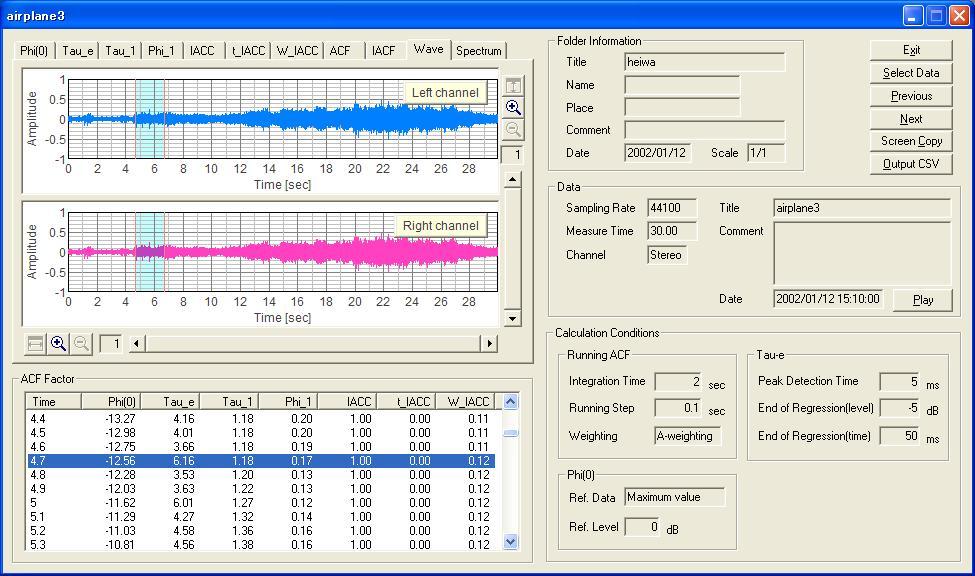
The next figure is the analysis result display. The graph shown is the temporal waveforms. The blue area indicated in the waveform display corresponds to the analyzed data portion listed in the ACF factor table. In this example, the area between 4.7 and 6.7 s is selected. The duration of 2.0 s is decided by the "Integration time".
I can see the temporal profile of the aircraft noise in this display. As the aircraft is approaching, the sound level increases from about 5s. It reaches the maximum at about 20 s and decreases again as the aircraft is receding. Also, I can hear a change in timbre of the aircraft noise throughout the recording. To evaluate this timbral change, I perform the spectrum and the ACF analysis at several points.
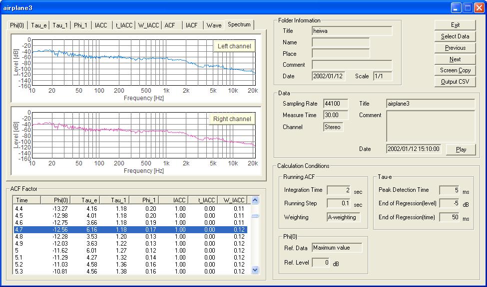
The next figure shows the spectrum of the data portion shown in the figure above. Note that the analysis is done with the A-weighting filter to consider the human ear's sensitivity.
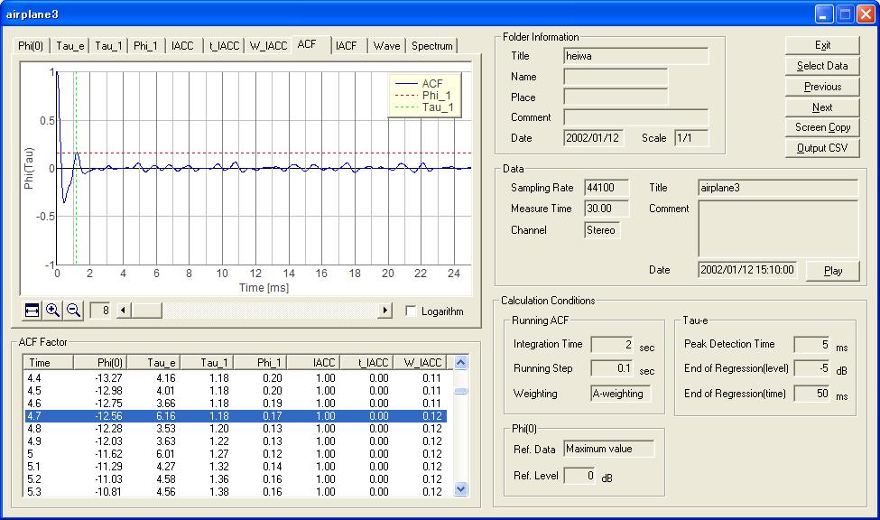
The next figure shows the ACF of the same data portion. The first peak in the ACF (tau_1) indicated on the graph corresponds to the representative frequency component. In this case, the tau_1 value is 1.18 ms as shown in the ACF Factor table below the graph. It means 1000 / 1.18 = 847 Hz.
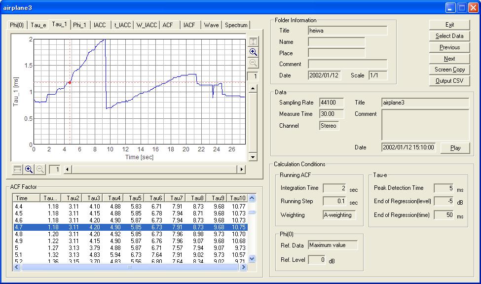
The next figure shows the time course of the tau_1 value. From this graph, I can see that the representative frequency decreases from 1250 Hz (1000 / 0.8 ms) at 0.8 s to 500 Hz (1000 / 2.0 ms) at 9 s. When I listen to the sound carefully, the sound changes at about 9 s. This change is reflected in the tau_1 graph. Other ACF factors can be analyzed similarly.
The acoustic analysis of noise in DSSF3 is proceeded as the following procedure:
1. Check the temporal waveform.
2. Use the oscilloscope to see the detailed waveform in real time.
3. Perform the FFT analysis, both in the spectrum and the octave band analysis, to see the frequency characteristics of sound.
4. Perform the ACF analysis to see the time change of the sound qualities such as pitch and reverberation. This is available in the Sound Analyzer. More information can be obtained than the conventional spectrum analysis.
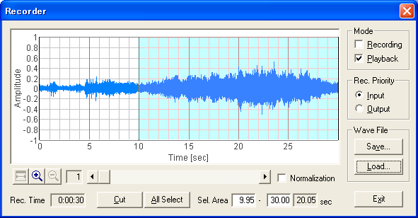
Next, the same sound (air2.wav) is analyzed by the spectrogram. The wav file is loaded on the recorder. To analyze only the meaningful portion of sound, the waveform is edited as follows.
First, right click on the waveform display and drag the mouse to select the portion to be remained. Only the selected portion will be shown as light blue.
Then, click the Cut button. Unselected portion (white background) will be cut out.
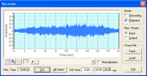
Now the data is ready. Let's start the analysis. Open the spectrogram, set the Time Range as 20 s, and set the Direction of Axis to Fwd. By clicking the Start button, the sound file will be reproduced and the measurement will start. Spectrogram will be drawn from right to left.
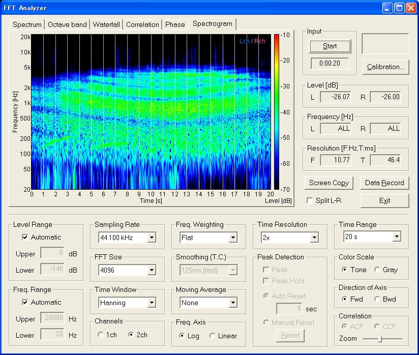
At a first glance, you may find that the high frequency energy is weaker than the previous landing sound. It may be reasonable because this sound is of airplane that is flying overhead. Also, it can be seen that no strong harmonics exist in this sound. Perhaps the high frequency tonal sound is attenuated when the sound passes the air, and only the relatively low frequency noise components remain. This analysis was done with the Flat frequency weighting. If it is analyzed with the A-weighting filter, high and low frequency energies will be more attenuated.
Spectrogram is a powerful tool for seeing the time series of spectra. The energy at a given time and frequency is displayed as a color map in a two dimensional diagram. Spectrogram is widely used in the speech analysis, bioacoustics, and other applications. Combination of the spectrogram and other functions, such as the power spectrum will be the most convenient way for identifying the important point of the sound.
January 2002 by M.Sakurai