| Japanese | English |
New analysis results by the latest version of DSSF3 is added to the original report written in January 2002.
Original report written in 2002
Measurement of landing aircraft noise at night in the residence area.
| Date: | 28 Jan. 2002 20:30 |
| Weather: | rain and snow mixed |
| Temperature: | 6 degrees centigrade |
| Humidity: | 60 % |
| Place: | Southeast of Nagoya Airport. In front of a restaurant (Located at point 3 shown in map below) |
| WAVE file: |

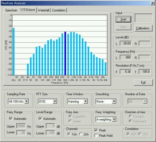
The lasting time of noise is short, since it passes at high speed compared with measurement near a runway. The following figure shows 1/3 octave analysis of noise. The levels are shown as the relative level, because the microphone is not calibrated yet. The sound level meter reading was 95dBA.
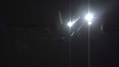
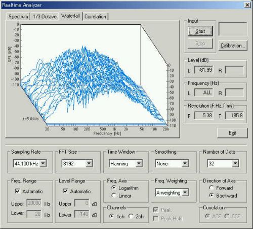
Three dimensional TEF (time-energy-frequency) display near the peak of the sound level
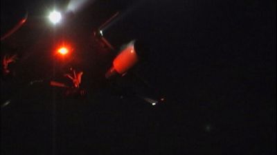
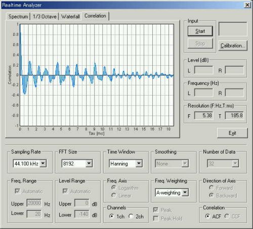
The real-time ACF display for the same portion.
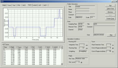
The running ACF measurement window.
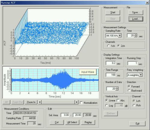
In the figure above, change of the sound pressure level is large from 9 to 14 sec after the measurement starts. According to the sound level meter, the level difference is 15dB (between 78 and 93 dB).
Analysis by the SA (Sound Analyzer)
Running ACF is calculated with the integration time of 2 seconds. It took 3 minutes even by the latest computer.
F(0): Relative sound pressure level
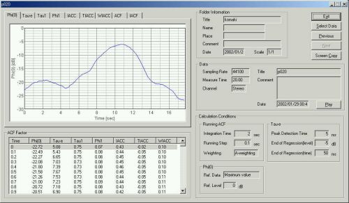
The maximum level appears at 11 s. The slope of the sound level is steeper than the previous measurement at the landing point. Level difference was similarly 15 dB in the previous measurement, but it went up gently in 5 seconds at first, and fell in 3 seconds later.
te
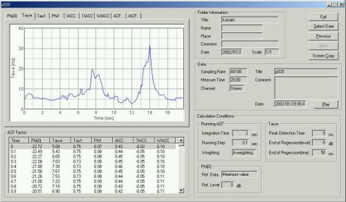
Effective duration of the ACF is around 5 ms during approaching. Compare this graph with that of the sound level. The value of te increases immediately at 8 sec with increasing sound level. Then it decreases to the minimum at the point with the maximum sound level. After that it reaches maximum again at 14 sec at which the sound level finishes decreasing. Finally it decreases to 5 ms again. This time change of te is same as in the previous measurement.
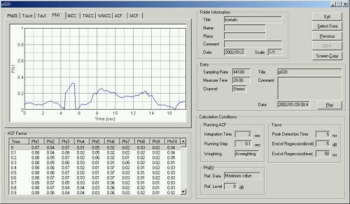
t1

The fundamental frequency of sound is expressed by t1 of the ACF. The value of t1 corresponds to the perceived pitch of sound so that t1 increases when the pitch decreases. The above figure shows that the pitch of the landing noise ranges between 700 and 1000 Hz, and it varies during passing through.
f1
The value of f1 represents perceived pitch strength. As typical cases, f1 for pure tone and white noise is 1 and 0, respectively. The above graph shows that airplane noise has weak pitch sensation in general. However, in the middle of the measurement time, at which the airplane is just above the head, f1 exceeds 0.2. For the sound with f1 above 0.2, we hear mixture of tonal and noise components, and that sound is actually very annoying.
IACC: inter-aural cross-correlation
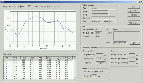
The measurement point is special this time, so that the jet plane passes through from left forward to right rear. When the body is ahead of a microphone, the value of IACC becomes large.
tIACC: inter-aural time difference
The angle of a microphone and a sound source is expressed. It will become zero if a sound source is in the front of microphones.
January 2002 by M.Sakurai
From here, written in 2004/08/11
First, I listen to the sound file air3.wav loaded on the running ACF window.

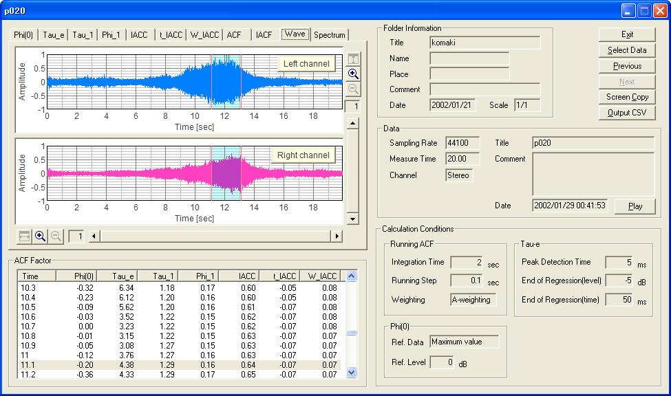
I think that this is a clear recording. The aircraft is just before landing to the runway. Because the measurement point was hidden by the residences, the sound becomes weak at once at about 5 s. The sound again increases from about 6 s as the aircraft approaches, reaches the maximum at 12 s, then decreases as the aircraft recedes. Here, I noticed a noise at about 16 s. To check this noise, I zoomed up the waveform display x32.
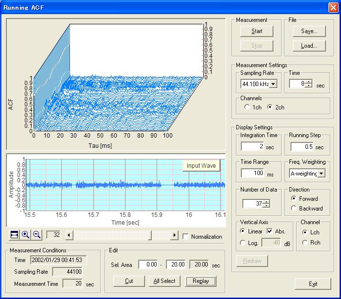
From the figure above, I can see small gaps in the data at 15.64 - 15.65 s and at 15.91 - 15.96 s. For further analysis, I cut this portion.
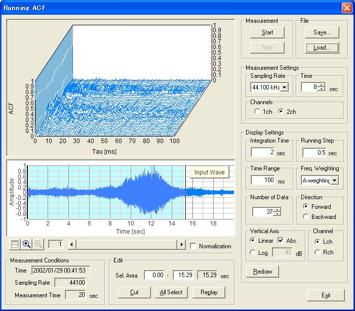
In the waveform display, right click and drag the mouse to select a data portion. The selected are is shown in blue. In this example, I selected from 0 to 15.2 s of data. Then click the "Cut" button to eliminate a non-selected area.
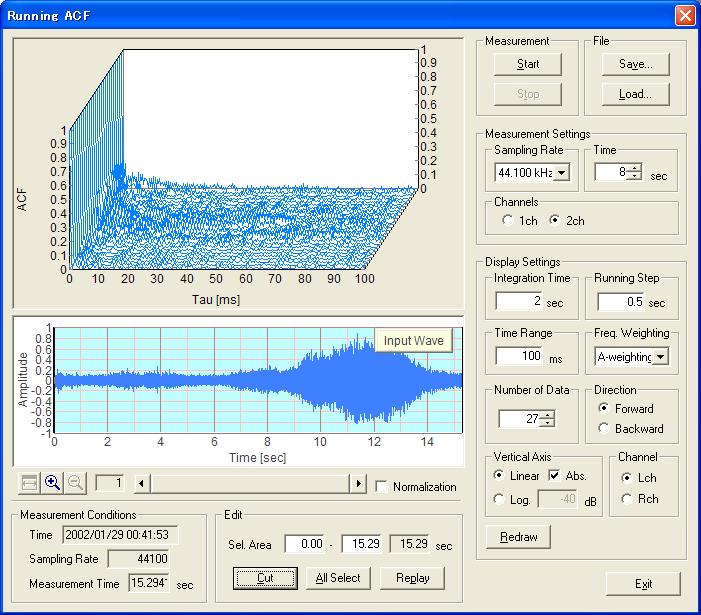
The sound data was edited as shown in the figure above. Now I start the analysis in SA. I saved the data on the Running ACF window by click the "Save" button. The "Save Measurement Data" dialog appears.
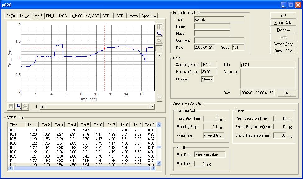
The next figure is the analysis result display in SA. The temporal waveforms of the aircraft noise are shown. The blue area indicated in the waveform display corresponds to the analyzed data portion listed in the ACF factor table. In this example, the area between 11.1 and 13.1 s is selected. This portion is the point at which the sound level is the maximum. The duration of 2.0 s is decided by the "Integration time". Double click a point in the waveform to select the analysis data frame.
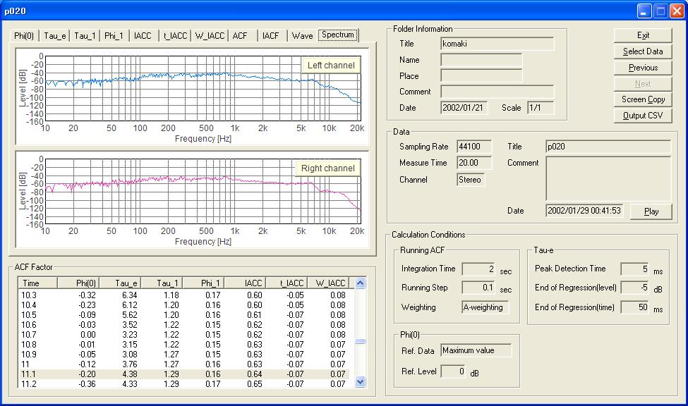
The next figure is the spectrum of the data portion selected above. I can see the maximum peak at 800 Hz (-40dB). This noise contains a wide range of frequencies from 25 Hz to 7 kHz within 20 dB.
The next figure is the ACF of the same data portion. The first peak in the ACF (Tau_1: 1.29 ms) broadly corresponds to the peak frequency in the spectrum (1000 / 1.29 = 775 Hz). This figure is zoomed up to x8, but when I see all the portion of the ACF, periodical peaks are found at around 12-14 ms, 24-28 ms, and so. This is perhaps because of the low frequency components of the jet engine noise. Such low frequencies can't be found in the conventional frequency analysis. This is the advantage of the ACF analysis.
Note about the jet noise generation mechanism
Jet noise is generated on the boundary of the fluid blew off at high speed,
and stationary air. Each of turbulent flows becomes a noise source because of
its the viscosity. In the area near a nozzle, disorder of a turbulent flow is
fine and generates high frequency sound. In area distant from a nozzle on the
contrary, with reduction in the flow velocity, disorder becomes large and low
frequency sound is generated. Therefore, the sound generated by the jet engine
becomes the broadband random noise. Representative frequency of the jet noise is proportional to the outflow
speed in the nozzle, and in inverse proportion to the diameter of the nozzle.
The strength of noise is proportional to the eighth power of the outflow
speed. (Rererence: ISBN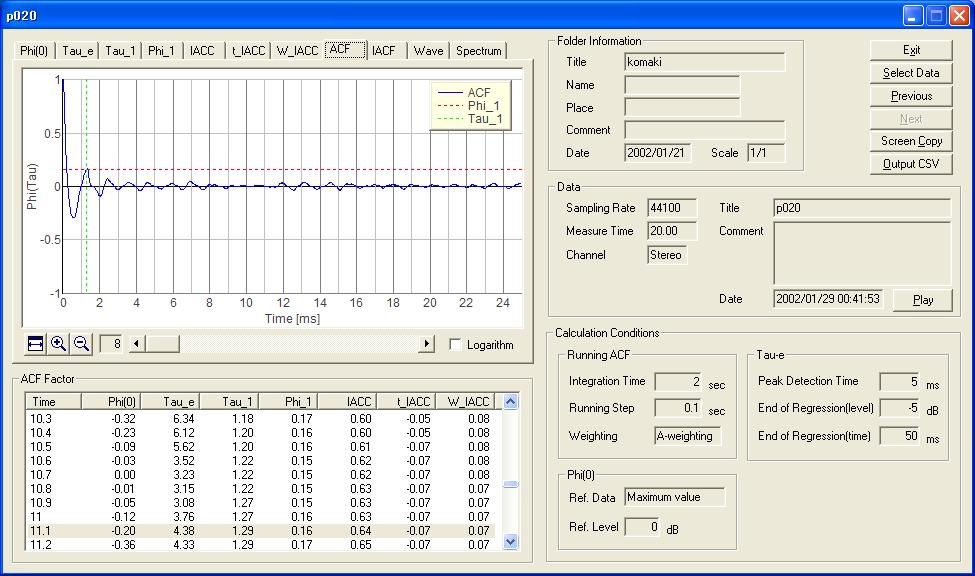
The next figure shows the time course of the tau_1 value. I can see that this value is increasing as the aircraft is approaching. It means that the representative frequency is decreasing, because tau_1 is the reciprocal of the frequency. This change in the representative frequency corresponds to the listening impression of sound. I assume that you notice that the pitch of sound is decreasing during the landing of the aircraft.
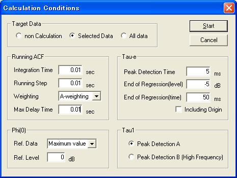
Next, I analyze the high frequency region of the same sound. For this analysis, the calculation conditions should be changed. The most significant parameter is the "integration time", by which the averaging time of sound is decided. The analysis described above was done with the integration time of 2 s, but now, it is set to 0.01 s.
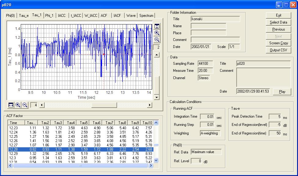
The next figure is the time course of the tau_1 value. It is clear that the values are smaller than before, though its fluctuation is large. The minimum value is 0.18 ms (5500Hz). It means that the aircraft noise contains higher pitch that is revealed by the high time resolution analysis.
The acoustic analysis of noise by using the ACF factor is a newly developed technology. You can find more information from Research, Paper and Presentation.
End of revision 2004/08/11