| Japanese | English |
New analysis results by the latest version of DSSF3 is added to the original report written in January 2002.
Original report written in 2002
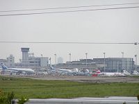
Noise from a fighter that takeoffs from the Air Self Defense Force Komaki base is measured this time.
| Date | 27 Feb. 2002 12:55 |
| Weather | Cloudy |
| Temperature | 18 degrees centigrade |
| Humidity | 48 % |
| WAVE file: |
  |
 |
Digital video camera (Sony Handy-Cam) and the external stereo microphones (Audio technica AT9450 one-point stereo condenser microphone) were used. It was recorded with videotape recording on a Mini DV tape with a 16-bit sound. By SONY VAIO DV gate-motion, iLINK connection was made and it reproduced. With Realtime Analyzer of RAE, a measurement screen was repeatedly reproduced, and the check of a measurement display was repeated.
Background noise was 48-50dB.
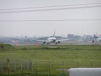
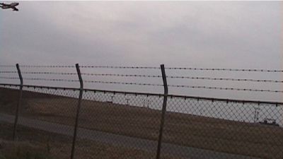
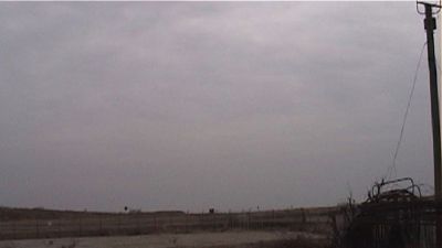
20:18There is a fighter on the upper left of the picture. It seems to
be the training plane T4 or F4 phantom.
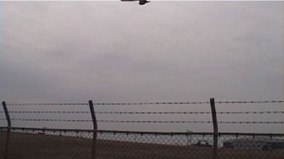
21:01
21:29
22:05
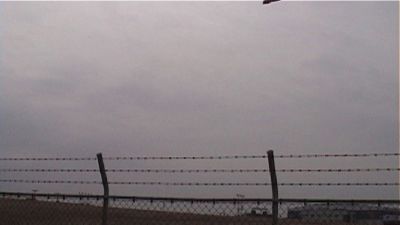
The above four pictures were cut from only 1.47 second. It was too quick to
follow up. Sound level was also large. It was measured by the sound level meter
as 118 dBA.
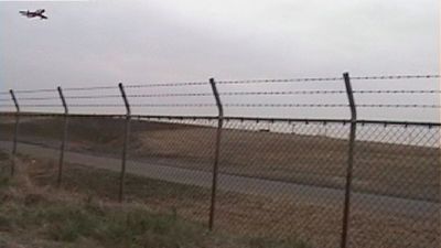
It is the angle of a vacant lot. It is just on the left of the first photograph.
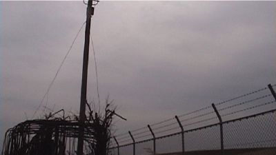
A runway is located in this direction. And the base of the Air Self Defense
Force is located on the left side.
The peak level meter display of a system without sound.
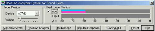
The background noise is analyzed. Sound level is about 49 dBA.
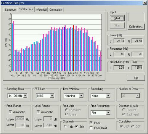
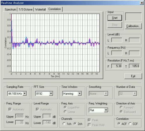
1/3 octave band analysis for the fighter noise
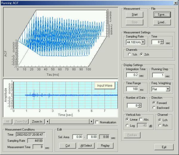
A characteristic real time autocorrelation display
The graph for the passenger plane landing is
resembled well.
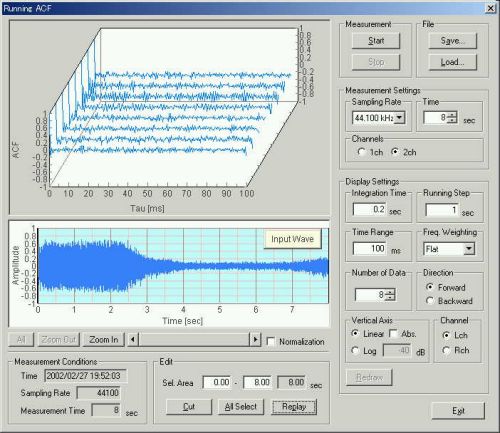
Running ACF measurement for 8 seconds. Integration time was 0.2 sec. The
graph below shows the sound waveform.
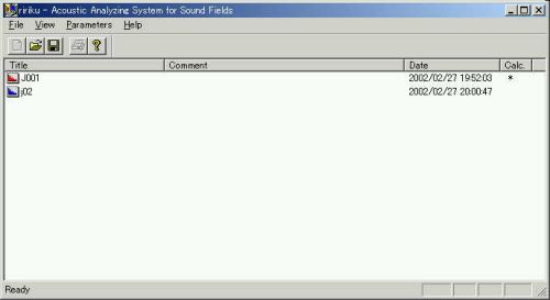
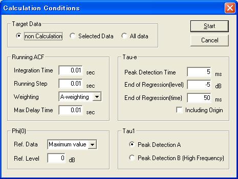
The files ware read on SA (Sound Analyzer).
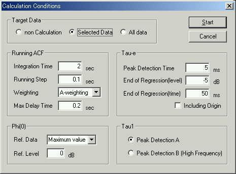
Calculation finished after 3 minutes with integration time of 2 sec.
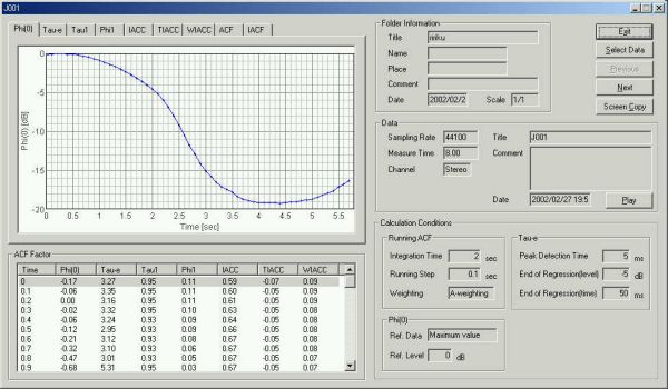
F(0): Graph of the time change of the sound level
Graphs of the time change for the analyzed values acquired from
autocorrelation and cross-correlation. You can save the graphs just by clicking the
"screen copy" button at the upper right of the analysis window.
When approaching, t1 is constant at 0.95
ms. It is the same as the landing passenger plane. When
going away, t 1 is 2.5 ms.
This low-pitched sound is probably caused by the exhaust sound.
The sound level meter recorded 118dBA just after passing through. As for jumbo jet, it
was 105dBA at the maximum.
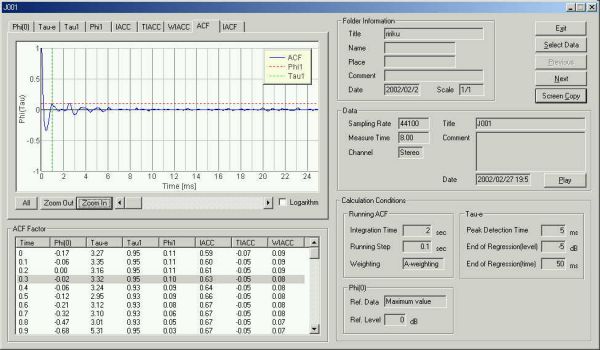
The ACF at 0.3 sec
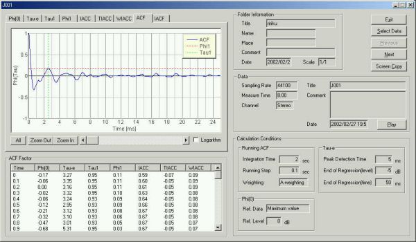
The ACF at 4.0 sec. You can see that the first peak of the ACF corresponds to
the fundamental frequency.
January 2002 by Masatsugu Sakurai
From here, written on 2004/08/12
First, I listen to the sound file air4.wav loaded on the running ACF window. Click the "Replay" button to play the sound. I use the headphones SONY MDR-200 for monitoring.
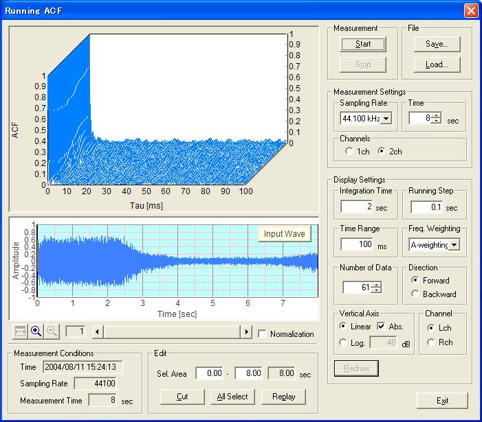
I think that this is a clear recording. The waveform shown in the figure above is the sound recorded in the left channel. At the beginning of the measurement, the jet plane suddenly took off. I measured the sound at the end of the runway. The plane passed just beside me from left to right at about 2 s. This is a very powerful sound. I felt a great shock wave when the plane passed. It is said that a car window glass would be broken by the shock wave of the jet fighter. The recorded sound cannot be comparable to the live sound, but I think that a secret of this powerful sound is contained in the recording.
Before the analysis, I checked the waveform by zooming up the display. There was a problem in the recording in the previous measurement. This time, I found no problem.
The data is analyzed with the following conditions. For analyzing the high frequency, the integration time should be short. Here, the integration time is set to 0.01 s. To mimic the human ear's frequency sensitivity, the A-weighting filter is used.
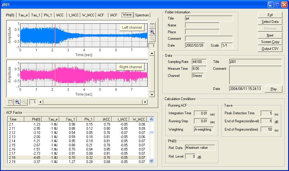
The next figure is the analysis result display in SA. The temporal waveforms in both channels are shown. The left channel input decreases and the right channel input increases from about 2 s. Now I can see that the jet passes from left to right.
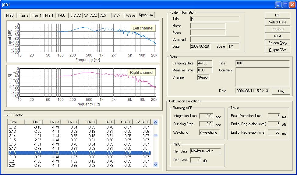
The next figure is the spectrum of the data portion selected above. I can see the peak frequencies at 350, 1.1k, 1.4k, 2k Hz, and so. This sound contains a wide range of frequencies
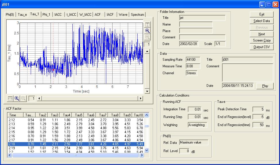
The next figure shows the time course of the tau_1 value. The tau_1 is the first peak in the ACF, that broadly corresponds to the peak frequency in the spectrum. The minimum value is 0.3 ms (3300Hz). It means that the aircraft noise contains higher pitch that is revealed by the high time resolution analysis. It is also seen that the pitch changes from high to low. This corresponds well to the listening impression of the sound.
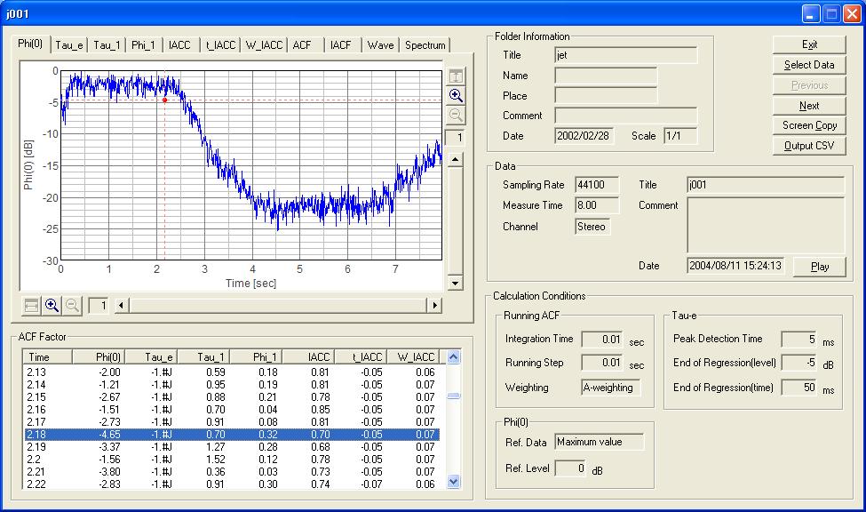
Next figure shows the time course of the sound level. The sound level is calculated as the averaged energy within the integration time. The envelope of the raw waveform is almost reflected in the sound level.
End of revision 2004/08/12