| Japanese | English |
revised on 2004/07/23
Since I wrote this measurement report, I learned that the cerebral infarction is caused by the heart disease, especially the heart failure. Blood will congeal, if its flow becomes irregular. If it occurred, the flow of blood in an artery supplying the brain is interrupted for longer than a few seconds, then the brain cells may die, causing permanent damage. I found out that it is important to supervise the motion of the heart which manages the blood flow to the brain in order to control so that an irregular pulse does not occur.
In this revision, the previous measurement is examined by using the latest version of DSSF3.
The original report written in April 2003
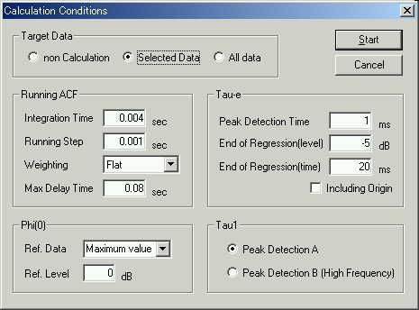
To increase the measurement accuracy of the timing of a valve movement less than 1ms, calculation conditions were changed. As a high temporal resolution,
heartbeat was analyzed with the integration time of 2 ms and the maximum time
delay of 20 ms in Heartbeat measurement 3. But I felt
at that time that this setting was too small. So this time, the maximum time
delay is set to 80 ms and the integration time is set to 4 ms. The running step
(1 ms) is not changed. Analyzed data is same as in Heartbeat measurement 5 and
6.
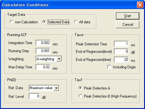
This is the calculation condition in this experiment.
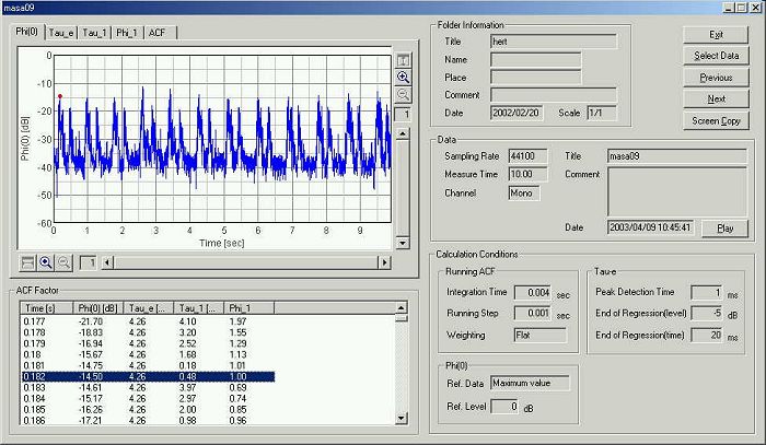
This is the time history of the sound level.
The time axis was zoomed up to X 8. The 1st and the 2nd sound of the first beat and the 1st sound of the second beat is displayed.
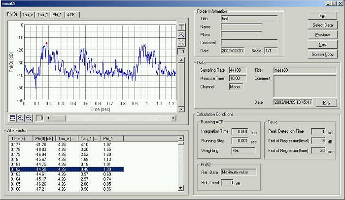
Phi_0 graph was zoomed up. Time course of the sound level for 1st and 2nd sound can be observed.
| Measurement time (s) | Phi(0) (dB) |
Tau_1 (ms) |
Phi_1 | Tau_e (ms) |
Comment | |
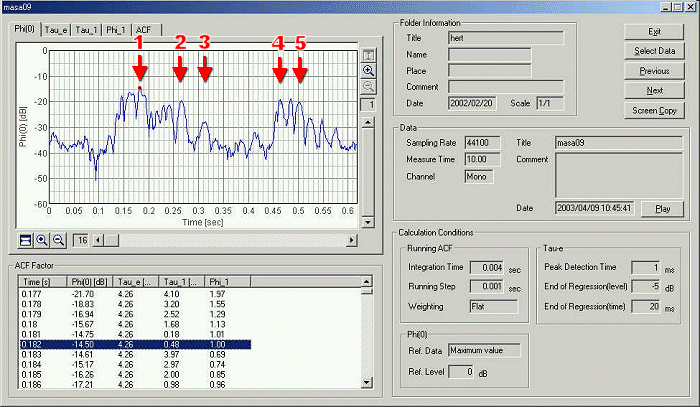
| 1 | 0.182 | -14.50 | 0.48 | 1 | 4.26 | Maximum sound level of the 1st sound. Closure of the mitral valve. |
| 2 | 0.265 | -19.58 | 0.75 | 0.99 | 108 | Second maximum of the 1st sound. Closure of the tricuspid valve. |
| 3 | 0.314 | - | - | - | - | Unknown |
| 4 | 0.464 | -19.04 | 2.28 | 0.23 | 2.28 | Maximum sound level of the 2nd sound. Closure of the aortic valve. |
| 5 | 0.502 | -20.25 | 0.68 | 0.99 | 16.69 | Second maximum of the 2nd sound. Closure of the pulmonary valve. |
Similarly, the timing of valve closure was measured for the second beat and the third beat. The measured values for each valve is summarized in the tables below.
Mitral valve
| Measurement time (s) |
Phi(0) (dB) |
Tau_1 (ms) |
Phi_1 | Tau_e (ms) |
| 0.182 | -14.50 | 0.48 | 1 | 4.26 |
| 0.976 | -15.35 | 0.27 | 1 | 14.24 |
| 1.783 | -15.06 | 4.42 | 0.73 | 1.43 |
Tricuspid valve
| Measurement time (s) |
Phi(0) (dB) |
Tau_1 (ms) |
Phi_1 | Tau_e (ms) |
| 0.265 | -19.58 | 0.75 | 0.99 | 108 |
| 1.059 | -20.18 | 0.63 | 0.99 | 10.02 |
| 1.865 | -20.36 | 0.07 | 1 | 6.05 |
Aortic valve
| Measurement time (s) |
Phi(0) (dB) |
Tau_1 (ms) |
Phi_1 | Tau_e (ms) |
| 0.464 | -19.04 | 2.28 | 0.23 | 2.28 |
| 1.265 | -18.70 | 0.05 | 1 | 2.26 |
| 2.067 | -18.73 | 0.05 | 1 | 8.94 |
Pulmonary valve
| Measurement time (s) |
Phi(0) (dB) |
Tau_1 (ms) |
Phi_1 | Tau_e (ms) |
| 0.502 | -20.25 | 0.68 | 1 | 0.99 |
| 1.295 | -20.30 | 0.77 | 1 | 1 |
| 2.102 | -20.57 | 0.07 | 1 | 1 |
It seems that a movement of the heart valve can be analyzed more precisely than
last time by setup of 4 ms integration time and 1 ms running step. The time
order of the valve sounds is constant (mitral -> tricuspid -> artery ->
pulmonary). The pitch of the valve sound changes abruptly at the moment a valve
closes. This is completely different from a sound with the fixed pitch.
April 2003 by Masatsugu Sakurai
From here, written in 2004/07/23
The same data is analyzed by the latest version of SA. The calculation conditions are shown below.
When I listen to the heart sound, I can imagine the movement of the heart valves like a spring. The duration of the valve closing sound is very short, and its level is quite small. But I think that the heart sound contains very important information expressing the state of the operation of heart valves.
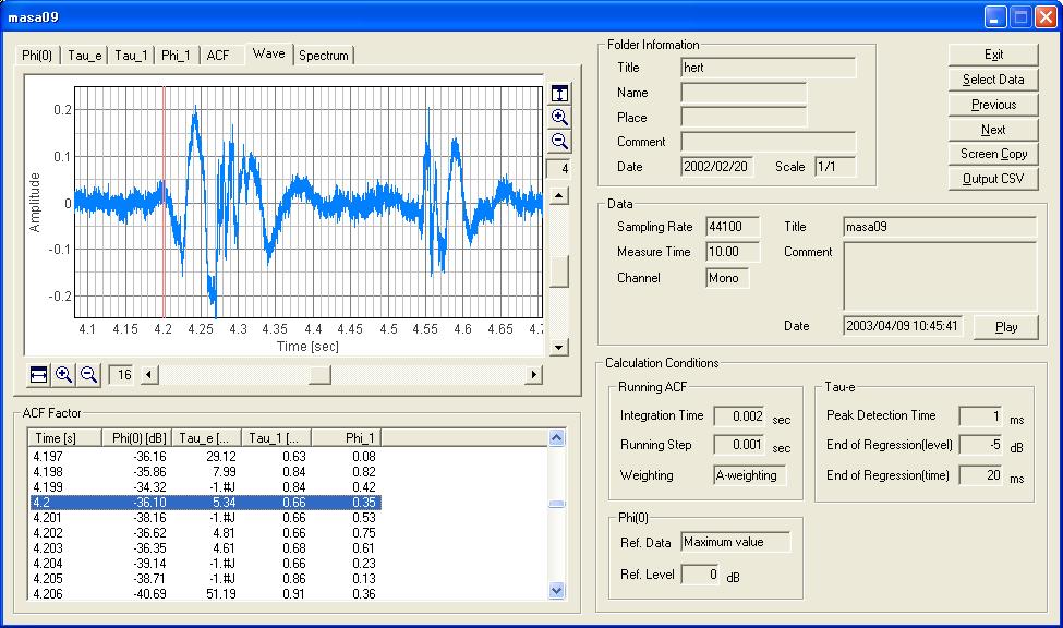
I set the integration time to 2 ms and the running step to 1 ms to analyze the timing of valve closure precisely. The next figure shows the time history of the sound level, focused on the portion of the first heart sound. The selected data portion is at 4.2 s, same as reported in Heartbeat measurement 6.
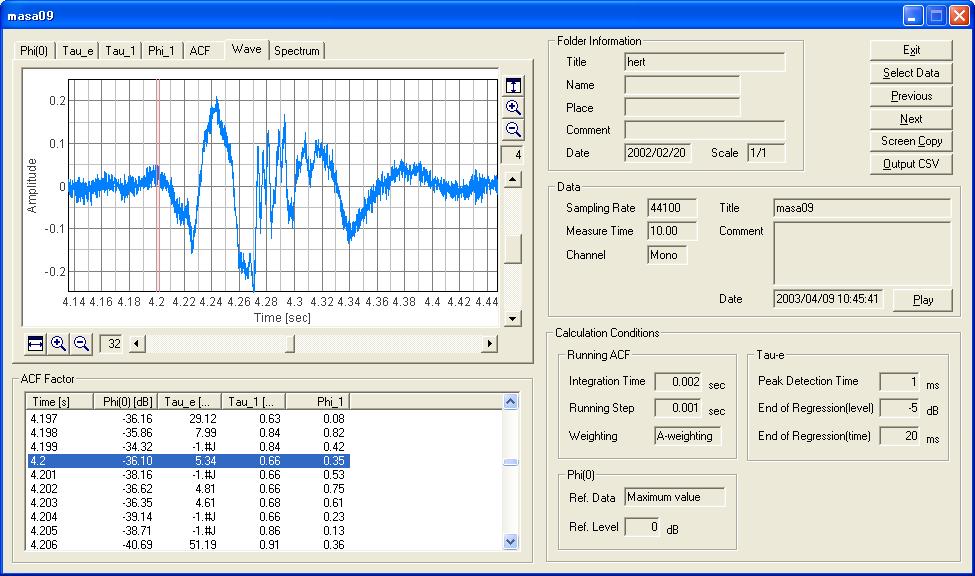
The same graph is zoomed up.
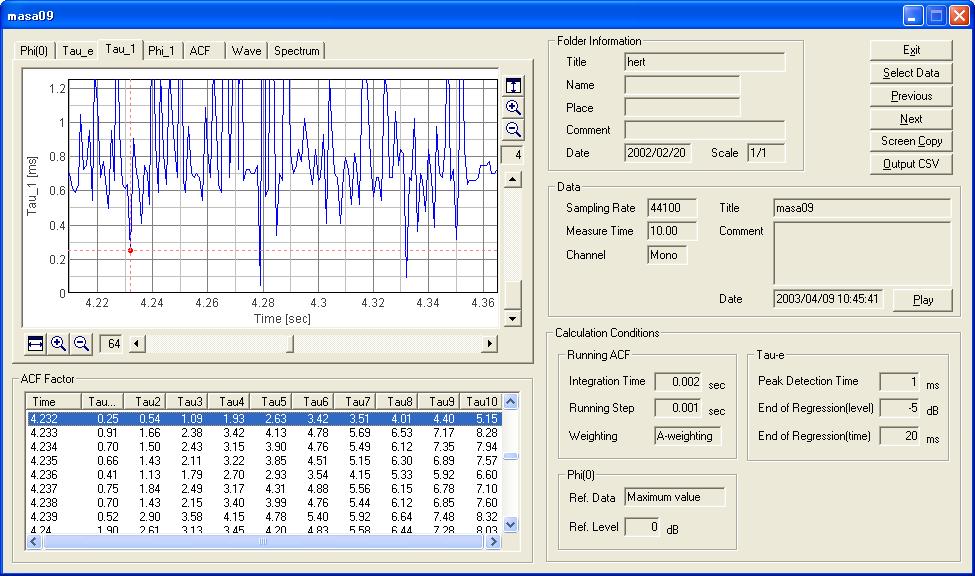
The valve closing sound should contain the high frequency component in comparison with the other continuous sounds. Now I check the time change of the Tau_1 value, which expresses the prominent frequency component.
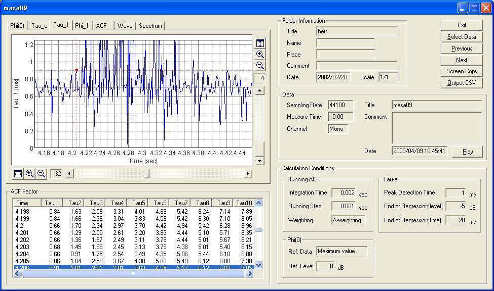
As expected, I can see the low values of Tau_1 (meaning the high frequency) at 4.23, 4.28, and 4.33 s. This portion of the graph is zoomed up in the next figure. You can see the minimum values of Tau_1 at three points as I mentioned. At these points, the peaks in the amplitude occur in the waveform display. These points probably correspond to the beginning of the valve closure.
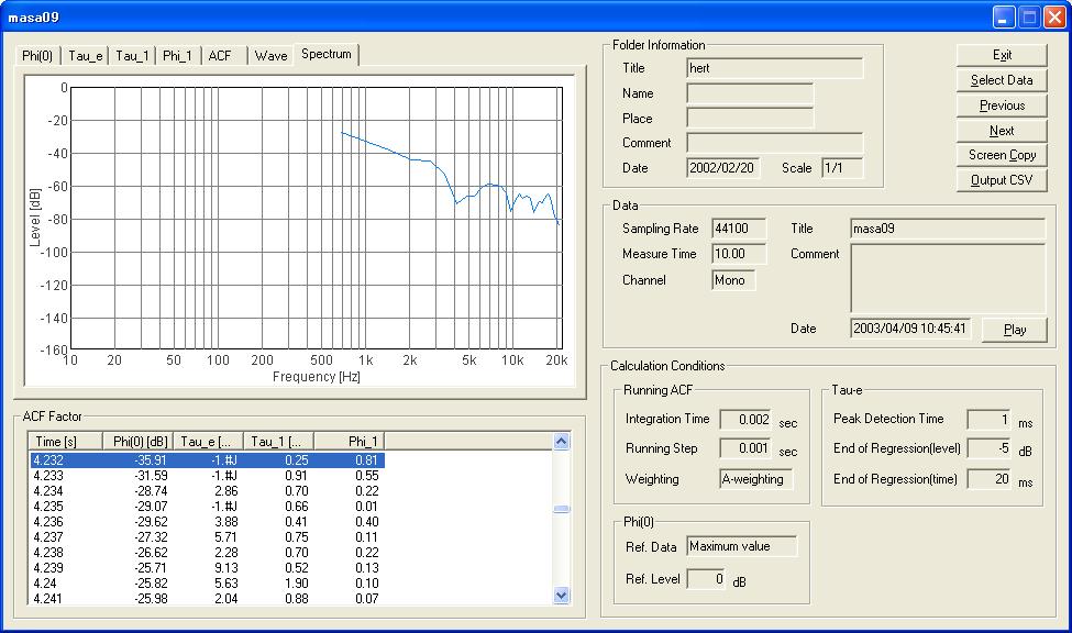
Because the integration time (analysis time length) is quite small, the frequency resolution is very poor. But you can see that the spectrum for this data portion contains high frequency peaks at 3 kHz, 7 kHz, and 18 kHz.
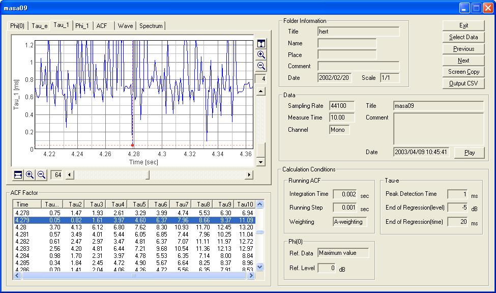
At 4.279 s, Tau_1 is 0.05 ms.
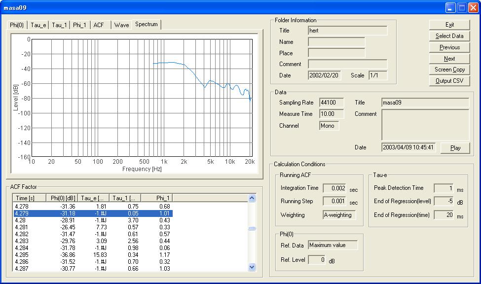
Its spectrum contains peaks at 5 kHz, 9 kHz, and 18 kHz.
In this report, I showed the spectrum analysis for a very short duration of the heart sounds using the latest version of DSSF3 (ver.5.0.5.6). I think that further sound analysis is possible if it is combined with other image processing data.
It has been said that the image analysis like a echogram is superior than the sound analysis. But I think it is not true. I think that the movement of the sound source (in this case, heart valves) can be analyzed from sound.
2004/07/23