| Japanese | English |
revised on 2004/07/22
The heartbeat measurement was first performed on February 2002. At that time, we wanted to know how the heartbeat is heard as music. However, it has been found that higher temporal resolution is needed to capture the characteristics of heartbeat and lung sound for the medical diagnosis. We went to the next step of biomedical sound analysis. Heartbeat measurement 1, 2, 3 are replaced by the new experiment in April 2003. In this report (Heartbeat measurement 5), it was explained how to record the heart sound using the stethoscope microphone.
Now I decided to analyze the same data again, because DSSF3 has been much improved since I wrote the first report. The results of the new analysis are reported in this page after the original report.
Heartbeat was measured again by a handmade stethoscope microphone. Microphone was stuck on the body with the gummed tape and care was taken not to make a noise. Subject stopped breathing. Heartbeat was measured by the running ACF measurement with monitoring a waveform. This measurement was taken at the same time with lung sound measurement 4.
| Date | 9 Apr. 2003 |
| Place | Home |
| Subject | 50 years old man |
| Microphone | SONY ECM-T150 Electric Condenser Microphone (Dimension: Diameter 6mm / Length 12mm) |
| Amplifier | SONY DAT WALKMAN TCD-D100 |
| PC | DELL INSPIRON 5000e |
| OS | Windows 2000 Professional |
| Software | DSSF3 |
| Other equipment | Stethoscope |
| Setup |  |
| WAVE file |
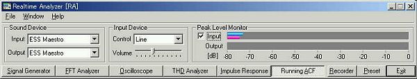
This is the peak level monitor at the time of no signal.
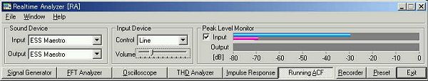
This is the background noise level measured with all equipments working and no input signal. It seems that the stethoscope microphone has high sensitivity. The level is between -28 and -35 dB.
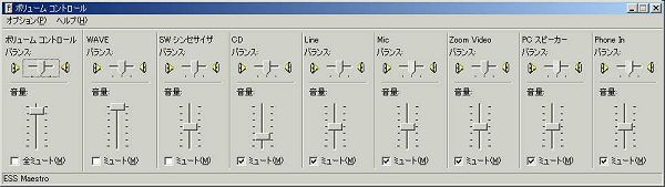
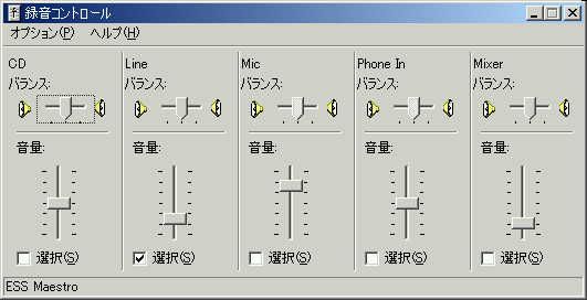
This is the Windows volume control. Devices other than WAVE is muted.
This is the recording volume control. Line is checked.
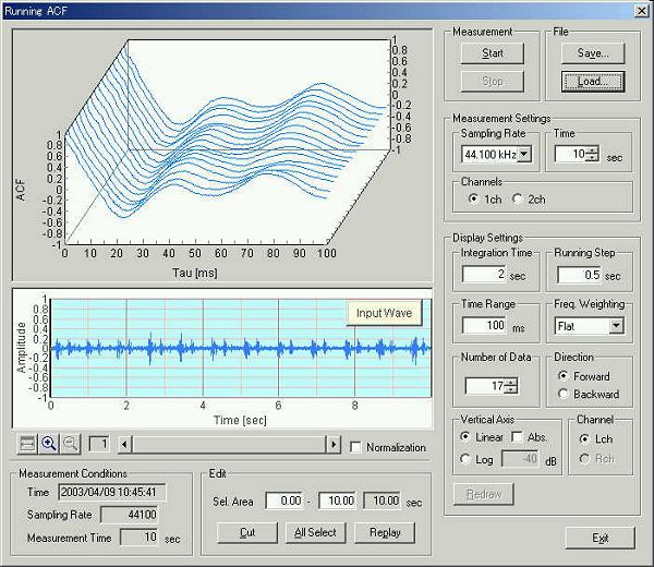
This is the running ACF measurement window. Click the Start button to measure the input signal from the microphone.
Then click the Save button. The "Save Measurement Data" dialog appears.
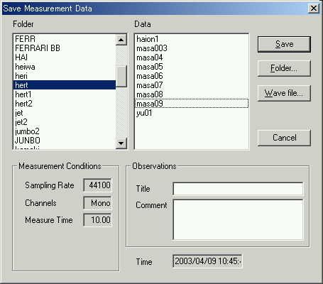
Measured data can be saved as the .wav format. The saved wave file here is a monaural data with 44.1 kHz sample rate.
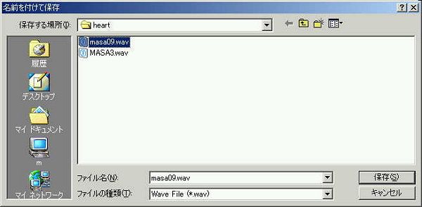
Wave file can be loaded from the running ACF window. Click the "Load" button and select the "Wave file". Sound file analyzed in this page is heart5.wav. Right click the link and save in the arbitrary directory.
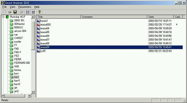
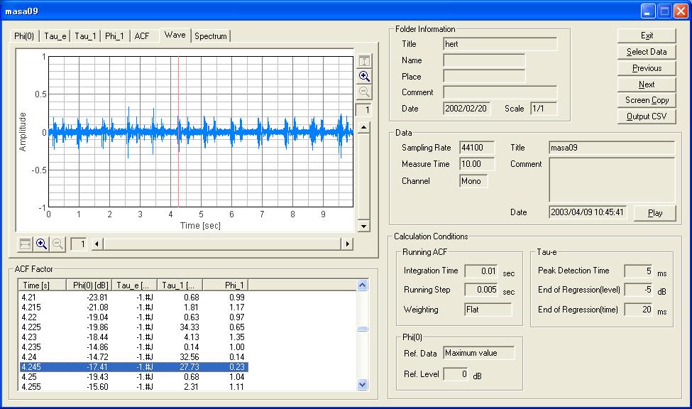
Start the Sound Analyzer (SA). In the main window, saved data is loaded.
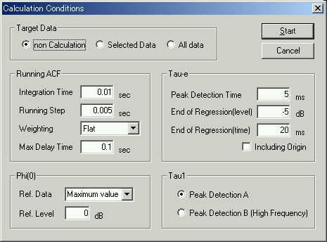
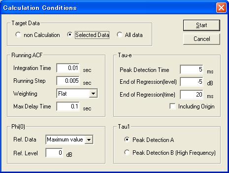
This is the calculation conditions window. Conditions are set for the high temporal resolution analysis.
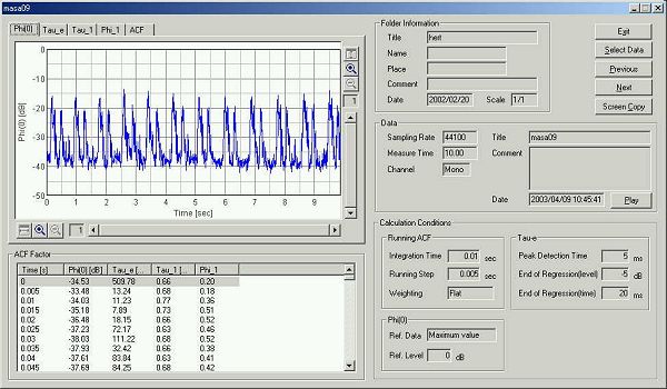
This is the analysis result screen. The Phi(0) graph shows the time history of the sound level.
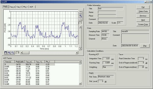
The graph above is zoomed in at the first 1 second.
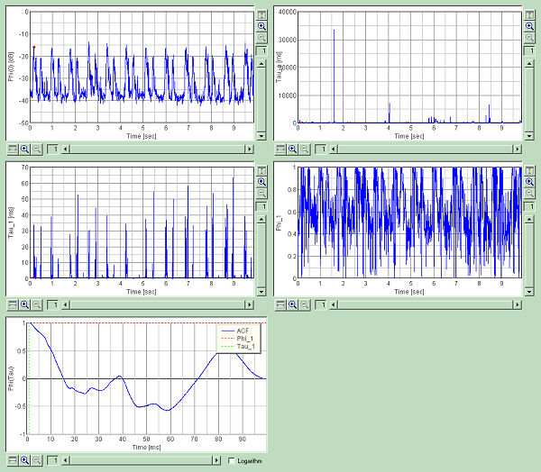
Time history of the acoustical parameters calculated from the ACF are shown below. This graph image is created by clicking the "Screen Copy" button.
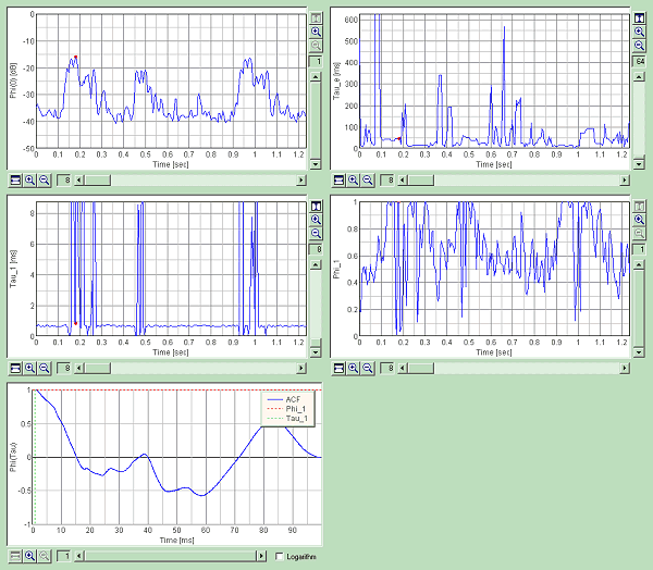
This is the time course of the ACF parameters for 10 seconds.
April 2003 by Masatsugu Sakurai
From here, written on 2004/07/22
The same data as above (heart5.wav) is analyzed by SA. Calculation conditions are set as below. This is the same setting as the original report.
This time, I show the analysis results by use of the new function in the
latest version of DSSF3 (ver.5.0.5.6), focusing on the temporal waveform of the
recorded heart sound.
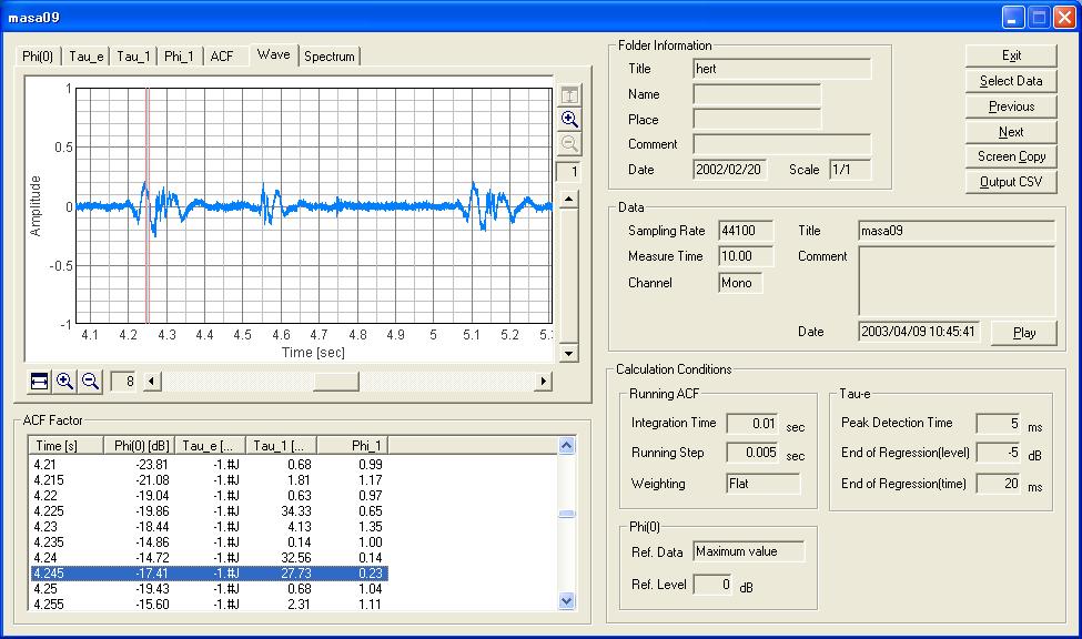
The next figure shows the temporal waveform of the recorded heart sound. Duration of the signal is 10 second. The sampling rate is 44100 Hz, so in total 441000 data is displayed. In the graph, the red line at 4.245 s indicates the analysis data frame chosen in the ACF factor table below the graph. By changing the graph tab, the spectrum or the ACF calculated for this data portion (whose duration is 0.01 s, set by the Integration time) is displayed.
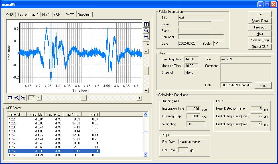
The next figure shows the temporal waveform of the same sound, that is zoomed x8 and focused to one cycle of heartbeat (from a first heart sound to a next first heart sound). The heartbeat rate is calculated from the interval of two successive first sounds. In this case, the interval is 5.105 - 4.242 = 0.863 s, and so the heartbeat rate is 60 / 0.863 = 69.5 beats per minute.
The next figure is further zoomed in to x16. The axis of the amplitude is also zoomed in. In the plot area, a first sound and a second sound are included. The interval between the first and the second sounds is 0.296 s. I can see that the first sound is louder than the second sound, and each consists of two successive peaks in the amplitude.
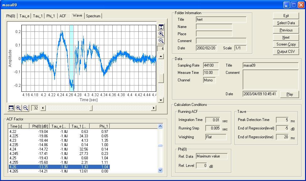
The next figure is further zoomed in to x32. Only one first sound is displayed. I can see that the the first sound begins at 4.2 s and end at 4.38 s. The duration of the first sound is 0.18 s.
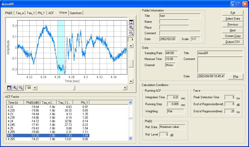
The next figure is zoomed in to x64 to observe the first sound in more detail. Y-axis is also zoomed up. We can see that the first sound consists of several separate components. Those components are caused by the closure of different valves. But when you listen to the sound file (heart5.wav), you can not decompose those components. That is because our hearing system integrates (averages) the incoming sound with some time constant. So, the sound pressure level is calculated by taking averages in the specified duration (in SA, the sound pressure level is calculated from the ACF). The time course of the sound level (in SA, it is called the Phi(0)) corresponds to the change in perceived loudness of sound.
2004/07/22