| Japanese | English |
Last updated on 2005/07/13
This measurement was originally performed in 2002/09, using DSSF3 ver.3, that is now sold as RAE version 2 since 2003/02.
The previous results are summarized as follows. It was found that Japanese vowel consists of at least two prominent frequency components. One is the fundamental frequency. The fundamental frequency is a rate of the vibration of the vocal fold. It is said that the fundamental frequency depends on the length of the vocal folds. It is about 150 Hz for male voice, is 250-300 Hz for female, and is higher for children's voice. The other is the formant frequency, that is caused by the shape of the vocal tract.
At the first measurement, DSSF3 did not have the high time resolution FFT analyzer that works with the ACF analysis. So, I estimated those frequencies by using the real time spectrum analyzer and the running ACF graphs separately. However, it took much time, and the time constant for the measurement might not be suitable for voice analysis. Since the FFT was performed on an arbitrary portion in pronunciation, it was lacking in reproducibility. These limitations did not allow me to investigate the voice quality appropriately. To overcome these limitations, DSSF3 has been improved as follows.
DSSF3 News 1
Jul 2003
Display of the Running ACF results [SA]
In the graph of analysis results, red mark is displayed on the specified point.
Now, it has been improved so that it is easy to treat a numerical data table.
Signal waveform and spectrum display are added [SA]
Temporal waveform and spectrum were added to the graph display of the ACF
analysis.
In the current version of DSSF3, the FFT analysis and the ACF analysis can be performed on exactly the same data. So, I decided to analyze the same data again. The results of the new analysis are reported in this page after the original report.
Original report written in 2003/04:
The fundamental frequency and formant frequency of vocal cords were investigated by the running ACF analysis.
| Date: | 17:00, 20 Sep. 2002 |
| Place: | Nagoya, Japan |
| Microphone: | SONY ECM-MS957 |
| Personal computer: | DELL INSPIRON 7500 |
| OS: | Windows 2000 Professional |
| Software: | DSSF3 |
| WAVE sound file: |
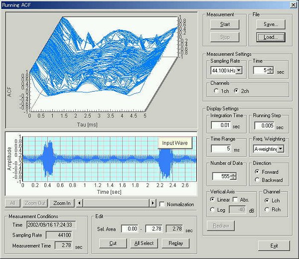
This is the running ACF analysis. A vowel "a" was uttered twice.
This is the power spectrum.
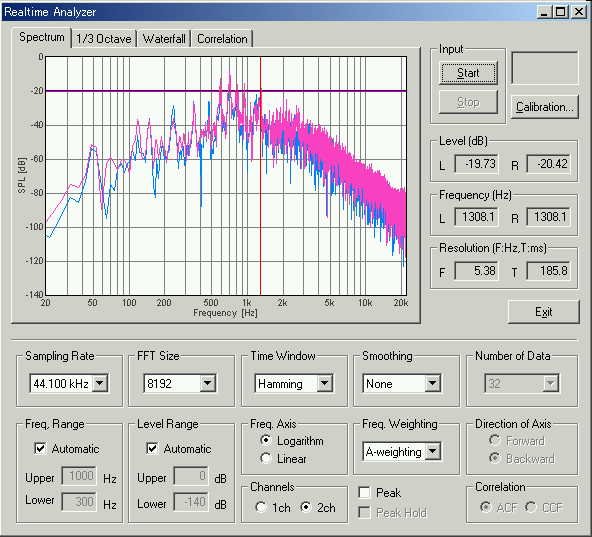
There are many peak frequencies in the spectrum, such as 48.4Hz, 118.4Hz, 150.7Hz, 236.9Hz, 355.3Hz, 484.5Hz, 597.5Hz, 650Hz, 716Hz, 834.4Hz, 958Hz, 1259.7Hz, 2799.3Hz, 3149.2Hz. In the time domain, those peak frequencies are found in the periodicity of the ACF. Reciprocal of the delay time of the ACF peak becomes frequency.
This graph shows the ACF waveform which was calculated for the integration
time of 10 ms and the analysis step of 5 ms. The analysis frame of this ACF is
same of the spectrum above.
In the figure above, the maximum peak is seen at 8.75 ms. This corresponds to the fundamental frequency of vocal tract, that is 114.3 Hz (1000/8.75).
Also, in the figure, the first peak is seen at 1.54 ms. This corresponds to 649 Hz and is called formant frequency.
It is said that the pitch of the vocal tract is almost fixed for vowel. In this analysis, the pitch was seen at 114.3 Hz. Although the voice pitch depends on a speaker or how to talk, it is fixed to some extent.
The pipe from a throat to a mouth and tongue determine a formant (resonance frequency), and determine a vowel tone. In the analyzed voice, the formant frequency was 649 Hz. From the formant frequency, the length of the vocal tract can be calculated as 34000(sound speed)/649(formant frequency)/4=13 cm. This also changes as the position of a tongue, but it is fixed for the same speaker.
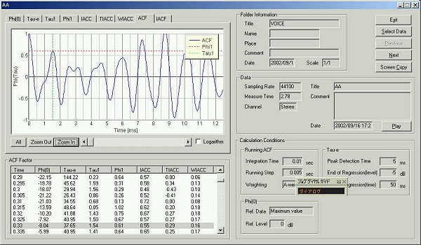
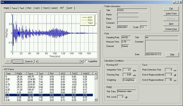
The same data is analyzed by the SA.
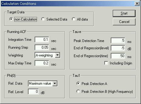
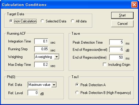
This is the calculation condition. The integration time and the running step
were set as 0.1 s and 0.05 s.
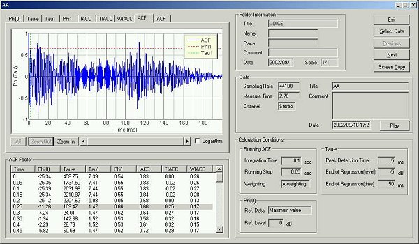
This is the result.
The ACF at 50 ms after utterance. The fundamental frequency is seen at 9 ms.
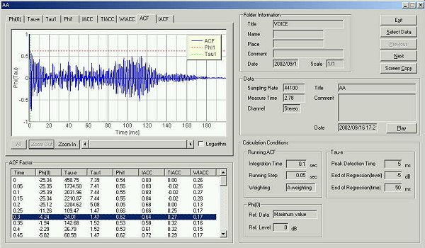
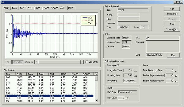
The ACF at 100 ms after utterance. The fundamental frequency is seen at 9 ms.
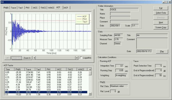
The ACF at 150 ms after utterance. The fundamental frequency is seen at 9 ms.
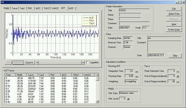
The ACF at 200 ms after utterance. The fundamental frequency is seen at 9 ms.
The ACF at 250 ms after utterance. The fundamental frequency is seen at 9 ms.
The ACF at 300 ms after utterance. The fundamental frequency is seen at 13
ms.
Next, the calculation condition is changed. The integration time and the running step was set at 10 ms and 5 ms.
This is the analysis result.
This time, vowel /a/ was analyzed by the running ACF in every 50 ms. It was found that the fundamental frequency and the formant frequency are clearly seen in the ACF waveform. Time change of these frequency components and their strengths becomes an important cue for identification of vowels. Also, the information about the length and the pitch of the vocal tract, which is extracted from the ACF waveform enable the identification of speaker. If it is analyzed in more time resolution, these information are obtained in more detail.
April 2003 by Masatsugu Sakurai
From here, new measurement report written in 2004/07/15
The same data as above A female voice data voice3.wav
is recalculated in SA with the same conditions. The integration time of 0.1 sec
and the running step of 0.05 sec are chosen.
(note: added on 2004/07/16)
I intended to report the analysis of data voice1.wav, but by mistake I analyzed voice3.wav reported in Analysis of the Japanese voice 3, since I have forgotten about the measurement at two years ago. So, keep in mind that this report is result of a female voice. If you are interested in male voice too, download voice1.wav and try the same analysis.
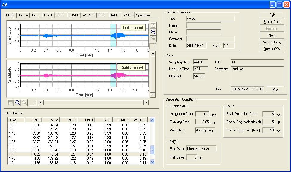
The figure below is the analysis result window. In the new version of SA, graph displays of Wave and Spectrum are added. The blue area indicated in the waveform display corresponds to the analyzed data portion listed in the ACF factor table. In this example, the area between 1.4 and 1.5 s is selected. The duration of 0.1 s is decided by the "Integration time".
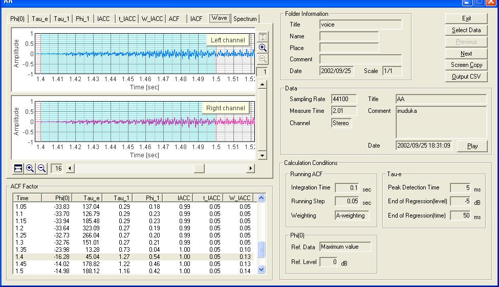
The next figure is the waveform display too, but now it is zoomed in to x16. This resolution has also been improved in the current version of SA. The measured data can be listened to by clicking the "Play" button in this window. Analysis results can be saved as a text data.
Next, I proceed to the spectrum display. FFT is also performed on the selected data portion indicated by the blue area.
The figure below shows the spectrum of data between 1.4 and 1.5 s. This portion corresponds to the first 100 ms after the utterance began.
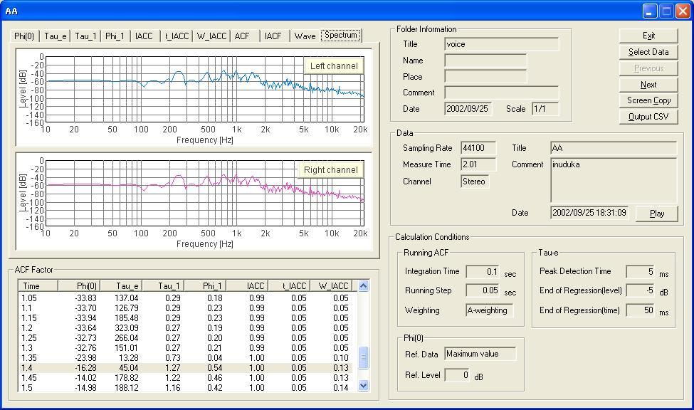
From this spectrum, we can see that the fundamental frequency is about 250 Hz. Formants are found at 750 Hz and 1kHz. Note that this spectrum is calculated for 100 ms of data. It means that the frequency components are averaged for 100 ms. If the actual voice changes more rapidly, this analysis is insufficient. Shorter integration time should be selected.
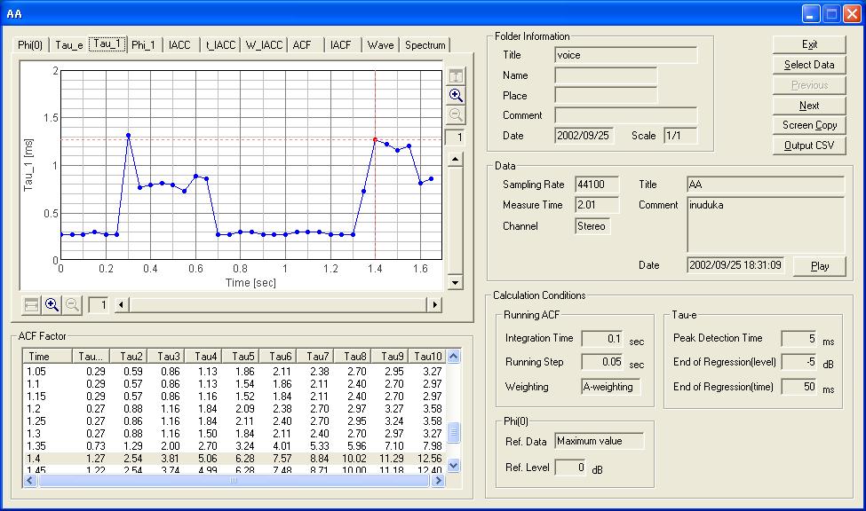
Next, I compare the spectrum with the ACF analysis. The figure below shows the time course of τ1 (first peak in the ACF), that corresponds to the formant frequency. At 1.4 s, τ1 is 1.27 ms , meaning 1000/1.27=787.4 Hz. This corresponds well to the formant read from the spectrum.
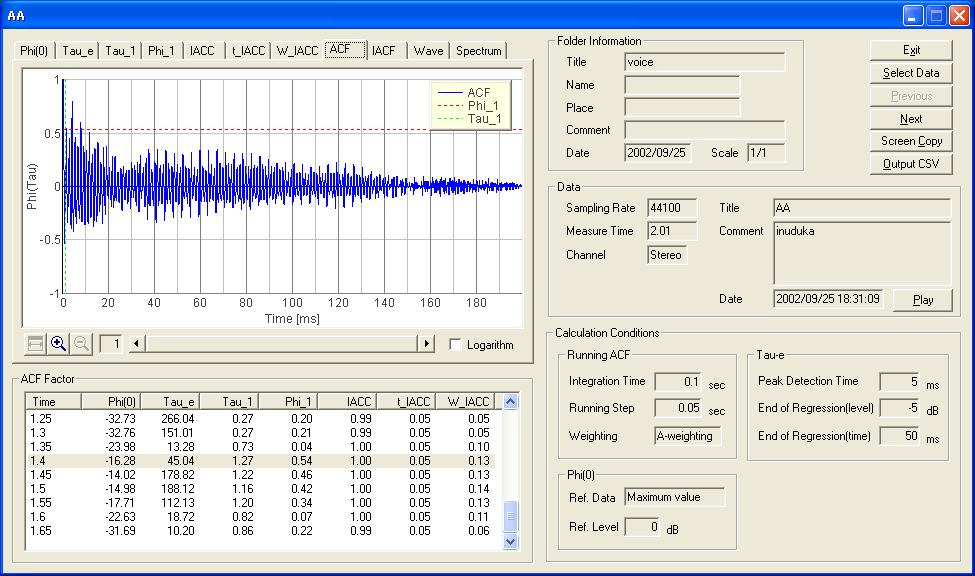
The next figure shows the ACF graph at 1.4 s.
I continue the analysis further.
From here, written in 2005/07/13
The same sound file voice1.wav was analyzed by the spectrogram (sonogram). Spectrogram is a representation of signal by time, frequency, and energy in a two dimension color map. Because most natural sound, like speech and music, is not stationary but varies over time, it is not sufficient to analyze one spectrum for the whole signal. Spectrogram is widely used in the speech analysis, bioacoustics, and other applications.
The wav file is loaded on the recorder. To play sound, "Playback" checkbox is marked. Rec. Priority is set to Input. This should be set to Output when the Signal generator's output signal is measured.
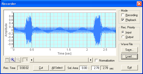
By clicking the Start button of the FFT analyzer, the sound is replayed and is analyzed until it ends. Time Range is set to 3 s to match the sound length, and Direction of Axis is set to Fwd. Other important settings are FFT size and Time Resolution. These parameters affect the time and frequency resolution of the spectrogram. Small FFT size results in finer time resolution and coarser frequency resolution, and vice versa.
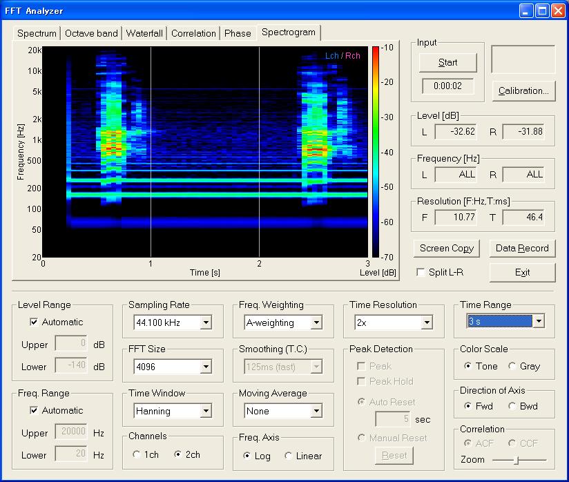
In the spectrogram, strong energy components are represented in green, yellow or red curves. These components correspond to the harmonics of speech sounds. The strongest two or three harmonics will be identified to formants. The lowest frequency peak is called the fundamental frequency (F0), and it corresponds to pitch of speech. Though it is masked by a hum noise, we can see F0s of two utterances at around 100 Hz. It seems that the second utterance has a lower pitch.
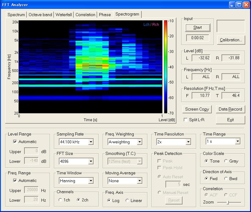
Next, the spectrogram will be zoomed in to the second utterance. By changing the Time Range setting to 1 s, only the second utterance was measured as below. It seems the time resolution is a little bit too rough yet. Try to increase "Time Resolution" parameter up to x8 and see how it looks. Also, try to change the Freq. Weighting to Flat. Lower frequencies will be emphasized.
Spectrogram is a convenient tool for visualizing sound. Temporally varying
frequency components can be clearly seen. This feature must be a valuable tool
for singing voice training, speech therapy, or measurement of voice quality. Of
course, any other kind of signals can be analyzed in the same way.
Masatsugu Sakurai