| TOP | STORE | DSSF3 | RAE | RAD | RAL | MMLIB | Support | Contact Us |
This reference manual is written for RA Version 2.0.0.1 and Version 3.1.6.8. Check the version of your RA (Help menu > Version information) before reading this document.
For users of Version 5.x.x.x, read the reference manual for Version 5.
Last updated: 2004/09/06
Last updated: 2004/05/24
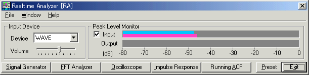
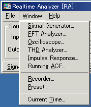
1-1. Menu bar
| Menu | Item | Description |
| File (F) | Exit (X) | Quit the application. |
| Window (W) | Signal generator (S) | Open / close the signal generator window. |
| FFT analyzer (F) | Open / close the FFT analyzer window. | |
| Oscilloscope (O) | Open / close the oscilloscope window. | |
| Impulse response (I) | Open / close the impulse response window. | |
| Running ACF (A) | Open / close the runnng ACF window. | |
| Preset (P) | Open / close the preset window. | |
| Help (H) | Version information (V) | Show the version information. |
| Read me (R) | Open the read me file. | |
| Online manual (M) | Open the online manual (only when connected to the Internet). | |
| Technical support (S) | Open the technical support page (only when connected to the Internet). | |
| Document Q&A (Q) | Open the Q&A page (only when connected to the Internet). | |
| Online update (U) | Execute the online update (only when connected to the Internet, and available only in Version 5.x.x.x.). |
*Alphabets after the item name ( _ ) show the shortcut keys.
1-2. "Input Device" and "Peak Level Monitor"
| Item | Description |
| Input Device | Selection of an input device. It is same as the Windows volume
control. [Example] Choose a "microphone" if your computer has a microphone input terminal and you want to use it. Choose a "line-in" if your computer has a line-in input terminal and you want to input a signal from external apparatus (e.g. DAT and pre-amplifier). When reproducing sound files (.wav) in signal generator or in Running ACF, choose WAVE or Mixer (this name depends on your computer or sound driver). |
| Volume | Adjustment of the input signal volume. Adjust the volume using peak level meter or an oscilloscope not to be distorted or not to be too small. |
| Input | Peak level monitor of an input signal. Check this box to start the display. |
| Output | Peak level monitor of an output signal. This level can be adjusted only by the digital volume in signal generator. When playing a wave file (in the Running ACF or the Impulse response), peak level of that file is displayed in real time. |
1-3. Function buttons on the main window of RA
| Buttons | Descriptions |
| Signal Generator | Tone, noise, sweep and pulse is generated as a stereo signal. As for tone, sinusoidal, triangle, square, and saw-tooth wave can be chosen. Each channel can generate different signals with specified frequencies. As for noise, white and pink can be chosen. Sweep is a tone signal of which frequency is varied continuously. Pulse signal is generated with specified number of time, duration and interval. |
| FFT Analyzer | Two channels spectrum analyzer, 1/3 octave band analyzer, 3D display (TEF), correlation function (auto- and cross-) can be chosen. |
| Oscilloscope | Two channels oscilloscope. |
| Impulse Response | The impulse response of a room is measured automatically with MLS (Maximum Length Sequence) or TSP (Time Stretched Pulse) methods. Measured impulse response can be saved as a wav. format. A wav. format impulse response can be imported from other measurement system. |
| Running ACF | The running ACF (autocorrelation function) and CCF (cross-correlation function) is measured. It is a time domain sound analysis method. Sound can be recorded up to 30 seconds. Recorded sound can be played and saved as a wav. format. A wav. format sound file can be imported. |
| Preset | Setup of RA can be stored as a "preset." Loading a preset, all settings of RA is recovered. Each preset is named and comment can be added. This function not only shortens the preparation time before the measurement, but it reduces a mistake. It is highly recommended to use this function for the easy and precise measurement. |
In the signal generator, several kinds of the test signals are generated automatically. Tone, noise, sweep, and pulse signals can be controlled and generated separately with an easy operation.
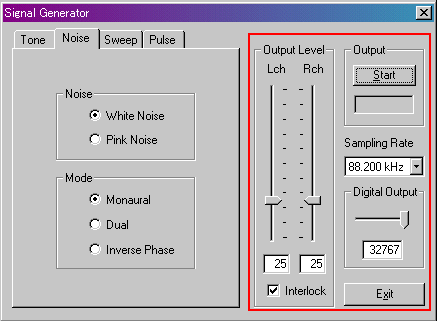
Common items in "Signal Generator"
| Name | Description |
| Output | The output of sound signals starts by clicking the [Start]
button. There is a stopwatch function. Time counter starts by clicking on the [Start] button and the time counter is displayed here during the output. The count lasts until the output is finished. |
| Sampling Rate | Number of sampling per second. Hardware is automatically checked and the available sampling rate is displayed. Generally, it is better to choose 44 kHz or 48 kHz. |
| Digital Output | Adjustment of the digital output level to pass through D/A converter. |
| Output Level | Adjustment of the analogue output level after the D/A converter. When the [Interlock] box is checked, left and right channels are outputted as the same level. This control is linked with the Windows volume control. |
| Exit | "Signal Generator" program finishes. |
Four functions of "Signal Generator"
| i. | Tone |
| The tone signal of sinusoidal, triangular, square or sawtooth waveform is generated at arbitrary frequency. | |
| ii. | Noise |
| The white noise or the pink noise are generated. | |
| iii. | Sweep |
| Sweep signal is generated with arbitrary start and end frequencies, sweeping speed and waveform. | |
| iv. | Pulse |
| The square pulse signal with arbitrary width and period is generated. |
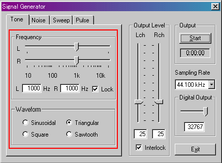
Explanation of the options in "Tone"
| Option | Description |
| Frequency | Specify a frequency by the numerical value or by the slider. When the [Interlock] box is checked, left and right channels are set equal. |
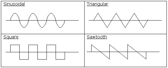
| Waveform | Choose the waveform of output sound from [Sinusoidal], [Triangular], [Square] and [Sawtooth]. |
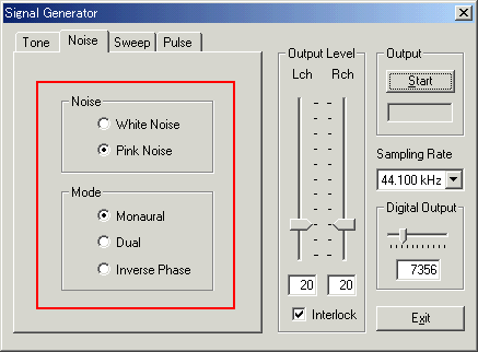
Explanation of options in "Noise"
| Field | Option | Description |
| Noise | White Noise | White noise contains equal energy for all frequency. Its power spectrum is flat. |
| Pink Noise | Pink noise contains equal energy for all octave frequency. Energy decreases for high frequency. Its octave band spectrum is flat. | |
| Mode | Monaural | Outputs the same signal for left and right channels. |
| Dual | Outputs a different signal for each channel. | |
| Inverse Phase | Outputs an inverse-phased signal for each channel. |
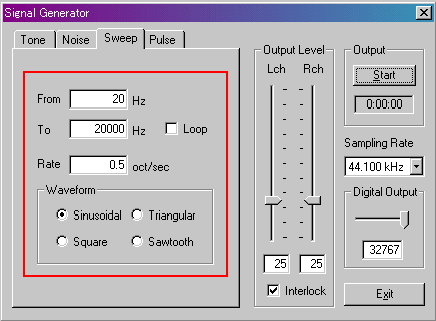
| Option | Description |
| From To |
The frequency sweep is generated from the frequency inputted in the [From] to the frequency inputted in the [To]. This is the logarithmic sweep, of which the frequency increases with a fixed rate of octave change per time. It means that the energy is constant within octave bands and it decreases at 3dB/oct. |
| Loop | Normally, a sweep signal is outputted only once. If [Loop] is checked, the output is repeated. |
| Rate | Sweep Rate [octave/sec]. |
| Waveform | Select the waveform of output sound. |
2-4. Pulse
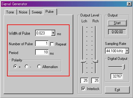
Explanation of the options in "Pulse"
| Option | Description |
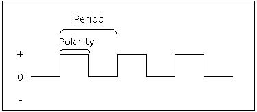
| Width of Pulse | Set up width of pulse [ms]. |
| Number of Pulse | The number of output. If [Interlock] is checked, the output is repeated. |
| Period | Set up a period [ms]. |
| Polarity | Set up polarity of a waveform.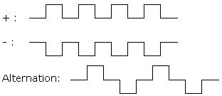 |
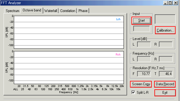
3. FFT Analyzer
In the FFT analyzer, 2ch spectum analyzer, octave band analyzer, TEF
(time-energy-frequency) analyzer, and correlation meter are available.
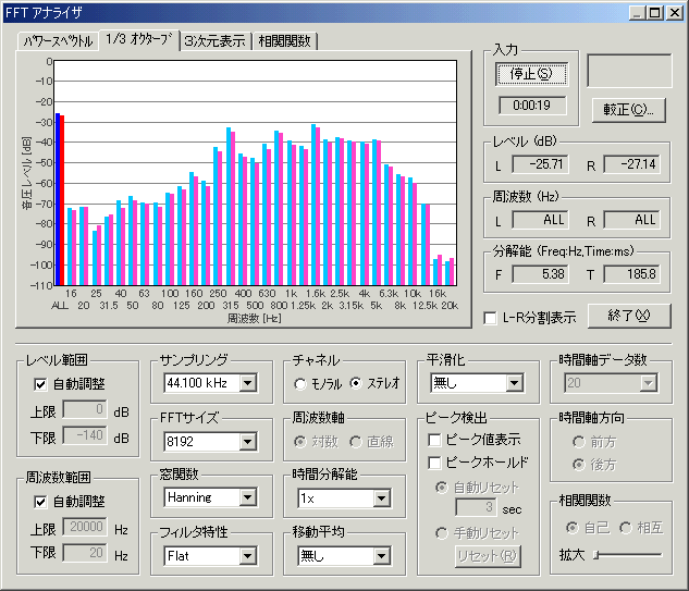
3-1. Common items of the FFT analyzer
| Commands or options | Descriptions |
| Input | Measurement starts with the [Start] button. Time counter starts when the Start button is clicked and the elapsed time is displayed here during the measurement. The time count lasts until the output is finished. |
| Calibration | The calibration of microphone are done. ->3-3. Microphone calibration |
| Level | Peaks of energy level for L (= left) and R (= right) are
shown respectively [dB]. By a left-click on the graph, the energy level at the frequency where you clicked on is indicated. By a right-click, the total level is indicated. |
| Frequency | Peaks of frequency for L (= left) and R (= right) are shown respectively [Hz]. |
| Resolution | Resolution is shown, which depends on a FFT size and a
sampling rate. F: frequency [Hz]. It shows the interval, at which the data is obtained. T: time [ms]. |
| Split L-R | If this checkbox is checked when the "2 ch" is selected, screen is split in two and data for each channel are displayed separately. |
| Exit | Finishes the "Realtime Analyzer". |
| Level Range | A setting of an indicated range of energy level (= vertical axis). |
| Freq. Range | A setting of an indicated range of frequency (= horizontal axis). |
| Sampling Rate | Set a sampling rate of A/D conversion. |
| FFT Size | A block size of FFT (Fast Fourier Transform). |
| Time Window | The time window is used to decrease extra frequencies,
Select the time window which meets the case. Rectangular: Rectangular window Hamming: Hamming window Hanning: Hanning window Blackman :Blackman window |
| Freq. Weighting | Select characteristics of auditory-filter from Flat, A-weighting, B-weighting, and C-weighting. |
| Channels | 1ch: One channel (light blue) 2ch: Two channels (light blue and red) |
| Freq. Axis | A setting of the scale on frequency axis. Logarithm: A rate is constant. Linear: A difference is constant. |
| Time Resolution | Speed of real-time display is specified. "1x" (standard), "2x" (double) and "4x" (4 times) can be specified as a refresh rate of a real-time display. |
| Moving Average | If the time is specified (1sec to 10sec, or until measurement end), The average value of specified period is displayed. |
| Smoothing | An indicated line is smoothed by averaging with a value
here. If the value is large, the line is easy to see, but the response is getting slower. |
| Peak Detection | Peak: A peak is indicated with blue (In the case of 2 channels, blue and red). |
| Peak Hold: Peak indication lasts for some seconds (Green). When "Manual Reset" is chosen, peak indication is done until the "Reset" button is pushed. When "Auto Reset" is chosen, peak indication is done during the specified period. |
|
| Number of Data | The number of time axes which are indicated in "Waterfall". |
| Direction of Axis | Direction of the time axis in "Waterfall". When [Forward] is selected, the time shifts forward on the screen. When [Backward] is selected, the time shifts backward. |
| Correlation | ACF: Autocorrelation is displayed. CCF: Crosscorrelation is displayed. Moving the "Zoom" slider makes it possible to zoom the correlation function to a suitable scale on time-axis. |
| maximize button close button |
3-2. Measurement windows
Five functions of the FFT analyzer| Items | Description |
| Spectrum | Measures the power spectrum of the input signal. Sound level is displayed as a function of frequency. |
| Octave band | Octave band analysis is performed. Energy at each octave band is displayed. |
| Waterfall | Time-energy-frequency analysis is performed. Results are displayed in the 3D graph. |
| Correlation | Auto- and Cross-correlation functions are measured. |
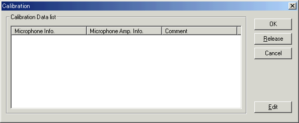
The Calibration dialog as below opens by clicking the Calibration button on the FFT analyzer. When the program is installed, no calibration data appears. To save a microphone data, click the Edit button.
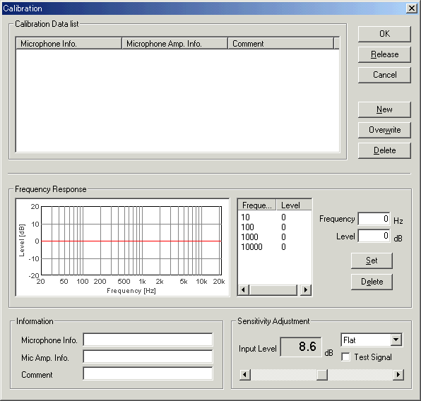
When the Edit button is clicked, the Calibration dialog expands and the edit window appears as below. On this window, the sensitivity calibration and the edit of frequency response curve are done. See the microphone setting in the operation guide for how to edit and save the microphone data.
The waveform of the input signal is observed. Vertical axis is amplitude and
horizontal axis is time. When "X-Y" check box is marked, horizontal
axis is left channel's amplitude and vertical axis is right channel's amplitude.
The mark ![]() on
the left of window indicates the point of trigger start level.
on
the left of window indicates the point of trigger start level.
Supplementary information of an oscilloscope New! 2004/01/20
The oscilloscope is generally used in checking an operation of electronic circuits. Voltage variations in a short time, or its oscillating waveforms are measured in real time. RA's oscilloscope not only measure the voltage waveform, but also waveforms of various signals through the input devices.
Input devices as below can be used by the oscilloscope.
| Device | Description |
| WAVE | Sound signal generated inside the PC, such as Windows Media Player or RA's signal generator, can be measured. |
| SW synthesizer(MIDI) | Output signal of the SW synthesizer can be measured. |
| CD player | Signal in the CD (test signal or music) can be measured. |
| マイク | Signal from the built-in microphones or devices connected to the microphone port can be measured. |
| telephony | Signal from the internal modem can be measured. |
| PCBeep | Phase difference between two channels can be measured. |
When measuring the voltage signal by using the electronic probe, the maximum input level of the sound mixer should be checked before the measurement. Usually, it ranges from 1.0 and 1.5 V.
The oscilloscope displays the input waveform as a digital value between -32767 and +32766. The values corresponds to the maximum voltage of the sound mixer.
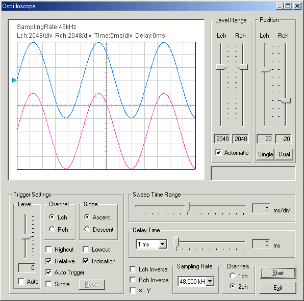
4-1. Items of the Oscilloscope
| Item | Description | |
| Level Range | Adjustment of amplitude (1 to 32768). There is [Automatic] function. |
|
| Position | A vertical position of a waveform is adjusted with a ruler for each
channel. If [Single] button is clicked, the waveform is arranged at the middle of window. If [Dual] button, two waveforms are arranged vertically. |
|
| Sweep Time Range | Time range for one graduation on the horizontal axis [ms]. | |
| Delay Time | An interval from the input to the display [ms]. Set the range of 'B', by selecting 1ms, 10ms, 100ms, or 1000ms from a pop menu (A). Then, adjust the delay time (= It is shown in the box 'C') with a ruler (B). For example, when you select "1ms" from a pop menu (A), The scales of a ruler (B) mean from 0ms to 1ms. When you select "10ms" in A, the scales of B mean from 0ms to 10ms. |
|
| Trigger Settings | Trigger settings are done here. | |
| Level | Trigger level is set up. This is the starting point of a waveform. There is an automatic adjustment function (Check [Auto] box.) |
|
| Channel | Select the channel which becomes the object of trigger settings. | |
| Slope | The timing of trigger. - Ascent: When a waveform gets over the trigger level in upward direction, the trigger is pulled. (A waveform starts upward.) - Descent: When a waveform gets over the trigger level downward, the trigger is pulled. (A waveform starts downward.) |
|
| Highcut | High frequency noise is cut. | |
| Lowcut | Low frequency noise is cut. | |
| Relative | With a check here, it is indicated relatively. Without a check, an absolute position is shown. | |
| Indicator | The starting level of trigger is indicated with " |
|
| Auto Trigger | If you check here, the indication is performed even when it has no trigger for a certain period of time. | |
| Single | Stops with the first indication. | |
| Reset | You can reset with [Reset] button, after you use [Single] function. | |
| Lch Inverse | Inverts a waveform of left channel up and down. | |
| Rch Inverse | Inverts a waveform of right channel up and down. | |
| X-Y | Indicates the left channel as a vertical axis and the right channel as a horizontal axis. It is shown with green. | |
| Sampling Rate | A sampling rate of A/D conversion. | |
| Channels | -1ch: One Channel(blue) -2ch: Left and right, two channels(blue and red) |
|
| Start (Stop) | Starts (and stops) an oscilloscope. | |
| Exit | Closes "Oscilloscope". | |
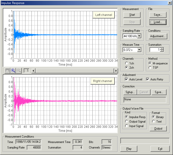
5-1. Items on the Impulse response window
| Field | Description |
| Measurement | The measurement starts with [Start] button. Though the measurement finishes automatically, you can stop it with [Stop] button. |
| File | [Save...] button: Saves the data measured here. -> 5-2.
Save measurement data [Load...] button: Loads the data stored previously. -> 5-3. Load measurement data |
| Sampling Rate | Sampling frequency. 8 to 48kHz. |
| Conditions | [Adjustment...] button: Input & output level, microphones position, measurement time are adjusted. -> 5-4. Adjustment |
| Measure Time | The time duration for measuring impulse response. (The scale on horizontal axis) |
| Summation | The number of times that MLS signal (period) are added and averaged out. If this number becomes larger, S/N ratio is improved. But, the time duration becomes longer. |
| Channels | Choose stereo (= 2 channels) or monaural (= 1 channel). |
| Method | The MLS method and the TSP method can be used in the impulse response
measurement. It can be used only by choosing one of the MLS and the TSP. TSP is the signal in which the energy of an impulse is distributed on the time axis. In the TSP method, an impulse response is calculated by generating TSP signal, acquiring the response and returning the dispersed energy. |
| Auto level | It is adjusted so that an output level can become the most suitable. (An
output level is enlarged within the range that an input doesn't become
saturated, and S/N ratio is improved.) If you turn "Auto Level" off. You can adjust sound volume (output level) at random using Windows sound volume control. |
| Auto Retry | Measurement will be repeated until distortion-free data can be obtained. You can release it at your option by switching on/off. |
| Correction | Unnecessary response of the measurement system such as microphone and
speaker are removed. [Setup...] button: Sets the Inverse filter. [Cancel] button: Cancels the Inverse filter. [Save...] button: Saves new Inverse filter. |
| Output Wave File | The data are saved in wave file format and text file format. |
| Play | Clicking on this enables to listen to the impulse response sound. |
| Exit | "Impulse Response" program is finished. |
| These buttons adjust the range of indication of impulse response. | |
| Measurement Conditions | Various conditions of the measurement are shown. (Time, Measurement Time, Bits, Sampling Rate, Summation, Channels) |
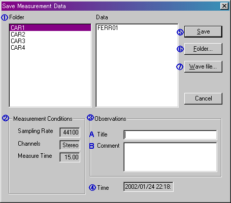
5-2. Save Measurement Data
Clicking [Save...] button on "Impulse Response" window, the following
"Save Measurement Data" window appears.
The measured data will be stored in a folder.
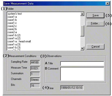
| No. | Field | Description |
| (1) | Folder | The folders, in which the measured data are stored, are listed. |
| (2) | Measurement Conditions | The measurement conditions of measured data are indicated. |
| (3) | Observations | Input the information about the data to save. |
| (3)-A | Title | Input data's name. |
| (3)-B | Comment | You can make optional comments upon the data. |
| (4) | Time | The time and date when data were measured. |
| (5) | Save | Saving is carried out. |
| (6) | Folder... | The folders in which the data are stored are managed. You can create new folder, alter the information such as folder's name, and delete a folder. ( -> Explained in the following section.) |
| 1. | Select the folder to save data; |
| From [Folder] list box , select the folder into which you want to save the measured data. If you want to save in a new folder, click [Folder...] button and create a new folder there. | |
| 2. | Input data's name; |
| Input the name of measured data into [Title] text box. And input the other information into [Comment] text box if necessary. | |
| 3. | Save the data; |
| Carry out with [Save] button. If you want to cancel, click [Cancel] button. |
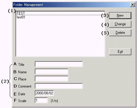
<Folder Management>
Clicking [Folder...] button on "Save Measurement Data" window, the
following "Folder Management" window appears.
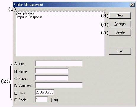
| No. | Button and Field | Description |
| (1) | - | The folders, in which the measured data are stored, are listed. |
| (2) | - | Information about the folder. |
| (2)-A | Title | Folder's name. |
| (2)-B | Name | The person who carried out the measurement. (Optional) |
| (2)-C | Place | The place where the measurement were done. (Optional) |
| (2)-D | Comment | Optional information. (Optional) |
| (2)-E | Data | The date when the folder was created. It is set automatically. |
| (2)-F | Scale | In the case of experiment with a model, its scale is inputted. For example, you measured the impulse response for 1/10 scale model, you should input "10" in the box. |
| (3) | New | Creates a new folder, which has the information you have inputted to (2). The new folder appears in the list box. |
| (4) | Change | Changes the information about the folder which is selected in the list
box. Select the folder in the list box, and the information about this folder are displayed in (2). Alter the information in (2) and then click this [Change] button. |
| (5) | Delete | Deletes the folder which is selected in the list box. |
Back to Items on the Impulse response window
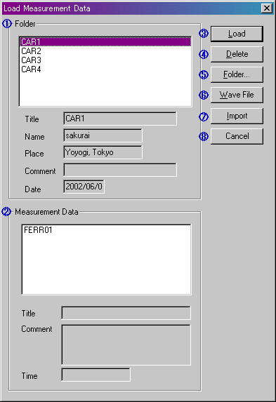
5-3. Load Measurement Data
Clicking [Load...] button on "Impulse Response" window, the
following dialog appears. Select the impulse response data you want to load,
here.
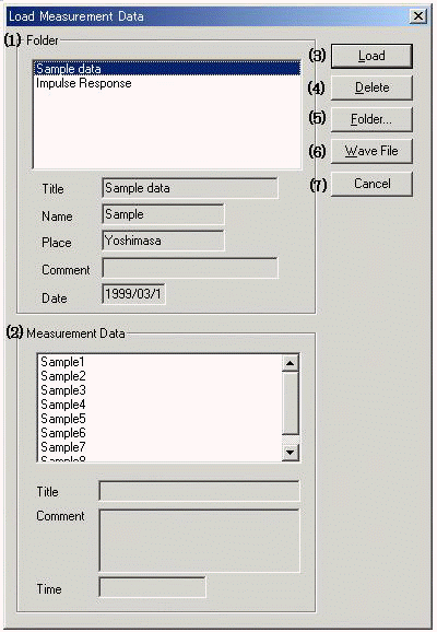
| No. | Field and button | Description |
| (1) | Folder | The folders, in which the measured data are stored, are listed. Here, select the folder which includes the data you want to load. The information (Title, Name, Place, Comment, and Date) about selected folder are shown below the list box. |
| (2) | Measurement Data | The data which are included in the folder selected in [Folder] list box
(1) are listed. Here, select the data you want to load. The information (Title, Comment, and Time) about selected data are shown below the list box. |
| (3) | Load | Loads the data selected in [Measurement Data] list box (2). |
| (4) | Delete | Deletes the data selected in [Measurement Data] list box (2). |
| (5) | Folder... | Opens [Folder Measurement] dialog. |
| (6) | Wave File | Loads wave file. |
| (7) | Import | Imports database of DSSF3/RAE/RAD. |
| (8) | Cancel | Closes this dialog without doing anything. |
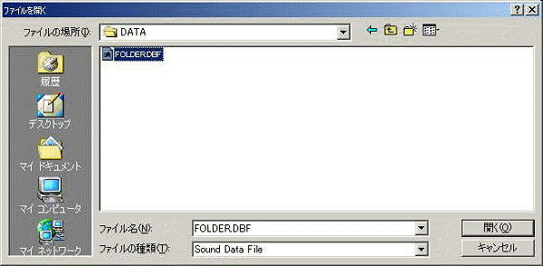
Database of the impulse response measurement can be imported from DSSF3/RAE/RAD on other PC.
Open the shared drive on your LAN.
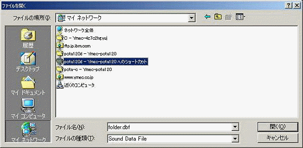
Open database of DSSF3.
Back to Items on the Impulse response window
5-4. Adjustment
Input and output level, microphone position, measurement time are adjusted
so that they can become the most suitable for the impulse response measurement.
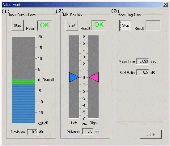
| No. | Field | Description |
| (1) | Input Output Level | By clicking [Start] button, a signal sound is outputted. Then, adjust
the volume of amplifier to the level marked with [Normal]. A result is indicated, "OK" or "NG". |
| (2) | Mic. Position | The difference between the distances from the sound source to left and right microphones is indicated in [Distance] text box. Adjust this value to "0". |
| (3) | Measuring Time | According to the size of reverberation in the sound field, the most
suitable time for measuring is set. When the measurement time is shorter in comparison with the reverberation time, the measurement is not carried out exactly. And, when the measurement time is too long, it takes long time to measure and calculate. |
Back to Items on the Impulse response window
5-5. Correction (inverse filter setting)
[Save] the inverse filter
In this window, the inverse filter is created from the measured impulse response. Only the initial part of the response should be selected because the response of the measurement system is included in this part.
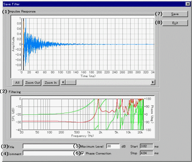
| No. | Fields | Description |
| (1) | Impulse Response | Measured impulse response is shown. The yellow area represents a
filtering range. Adjust the boundary of the yellow area, so as to include the part which is thought of as the impulse response of the measurement system within the yellow area. Drag left and right borderlines when the mouse cursor shape changes to "<-| |->" over borderline. |
| (2) | Filtering | Characteristics (Level, Phase) of the inverse filter corresponding to
the impulse response which is cut out from (1) are indicated. Red curve is characteristic of sound pressure level, and green curve is the phase characteristic. |
| (3) | Title | Input the name for the present inverse filter. |
| (4) | Comment | Input the comment on the present inverse filter. |
| (5) | Maximum Level | Sets the SPL limit for correction of the inverse filter. |
| (6) | Phase Correction | When this box is checked, both SPL and phase are corrected. If not, only SPL is corrected. Ordinarily, it should be checked. |
| (7) | Save | Saves the inverse filter. |
| (8) | Exit | Closes this dialog. |
[Setup] the inverse filter
To set the filter, click the "Setup" button and select the filter.
Then start the measurement. The impulse response of a room excluding the
response of the measurement system can be measured.
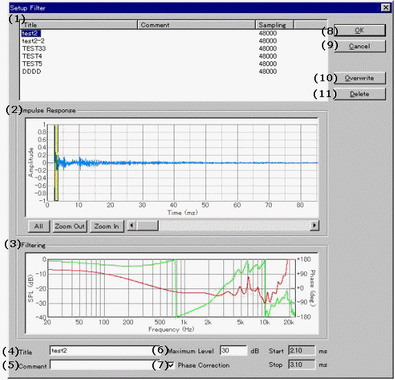
| No. | Field | Description |
| (1) | (List box) | The inverse filters which have been stored are listed. |
| (2) | Impulse Response | Measured impulse response is shown. The yellow area represents a
filtering range. Adjust the boundary of the yellow area, so as to include the part which is thought of as the impulse response of the measurement system within the yellow area. Drag left and right borderlines when the mouse cursor shape changes to "<-| |->" over borderline. |
| (3) | Filtering | Characteristics (Level, Phase) of the inverse filter corresponding to
the impulse response which is cut out from (2) are indicated. Red curve is characteristic of sound pressure level, and green curve is the phase characteristic. |
| (4) | Title | The name of the present inverse filter. |
| (5) | Comment | The comment on the present inverse filter. |
| (6) | Maximum Level | Sets the SPL limit for correction of the inverse filter. |
| (7) | Phase Correction | When this box is checked, both SPL and phase are corrected. If not, only SPL is corrected. Ordinarily, it should be checked. |
| (8) | OK | Applies the selected inverse filter to the measurement. |
| (9) | Cancel | Closes this dialog without doing anything. |
| (10) | Overwrite | Saves the altered inverse filter. |
| (11) | Delete | Deletes the selected inverse filter. |
Back to Items on the Impulse response window
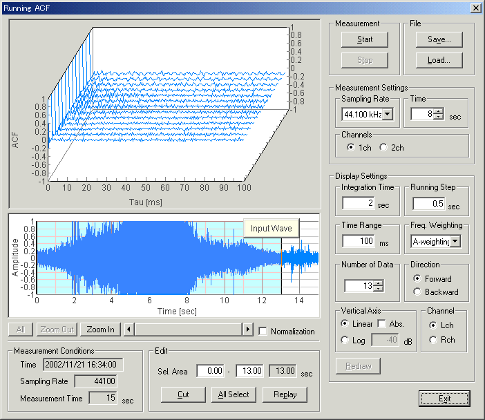
6-1. Items on the Running ACF window
| Items | Descriptions | |
| Graph (Upper) | The graph of the Running ACF is displayed. The vertical axis is the autocorrelation, the horizontal axis is the time, and the depth is the running step. | |
| Measurement | The measurement starts with [Start] button. Although the measurement stops automatically if the time you have set passes by, it is possible to stop it with [Stop] button. | |
| File | [Save...] button is used for saving the measured data in a file
(database) -> 6-2. Save
measurement data
[Load...] button is used for loading the stored data. -> 6-3. Load measurement data |
|
| Measurement Settings |
Sampling Rate | A sampling rate of A/D conversion. (44.1 or 48 kHz is recommended) |
| Time | Set the time for measuring. | |
| Channels | Choose the number of channel used for measurement, 1 channel (monaural) or 2 channels (stereo). | |
| Display Settings |
Integration Time | Set the Integration Time of ACF between 0.001 and 10 s. |
| Running Step | Set the Running Step (calculation interval) between 0.001 and 10 s. | |
| Time Range | Set the maximum value of the horizontal axis (t) in the graph. | |
| Freq. Weighting | Select the frequency weighting filter. | |
| Number of Data | Set the number of the data on the time axis (= The depth of graph) | |
| Direction | Set the direction of the time axis of the graph. Forward: The time shifts forward. Backward: The time shifts backward. |
|
| Vertical Axis | Set the scale of the vertical axis (Autocorrelation value). Linear: Autocorrelation is indicated in linear scale between -1 and 1. If [Abs.] box is checked, absolute value of Autocorrelation is indicated between 0 and 1. Log: Autocorrelation is indicated in logarithm (decibel) scale. Its range is from 0 dB to the value inputted to the right text box. |
|
| Channel | In the case of stereo measurement, left channel's data is displayed by checking "L ch" radio button, and right channel's data is displayed by checking "R ch" radio button. (Left channel's data is displayed in light blue, and right channel's one is pink.) In the case of monaural measurement, only left channel is displayed. | |
| Redraw | When the setting is changed, clicking on this button displays new data. | |
| Input Wave | The waveform of the input signal is displayed. | |
| Normalization | The input data is normalized between -1 and 1. | |
| Edit | Unnecessary part can be removed from the measured data. [Sel. Area] text boxes: Input the start and the end of the part you want to select. The selected area is painted with light blue. Or, this light blue area is changeable by dragging its left and right borderlines when the mouse cursor shape changes to "<-||->" over borderline. [Cut] button: Cuts off the part except light blue area. [All Sel.] button: Selects the whole area. (The whole area become light blue.) [Replay] button: Outputs the selected part (light blue area) from the speaker. During playback, a green line indicates where is replayed. |
|
| Measurement Conditions | The measurement conditions (Time, Sampling Rate, Measurement Time) are shown. | |
| Exit | Finishes "Running ACF" program. | |
6-2. Save Measurement Data
Clicking [Save...] button on "Running ACF" window, the following
"Save Measurement Data" window appears.
The measured data will be stored in a folder.
| No. | Field | Description |
| (1) | Folder | The folders, in which the measured data are stored, are listed. |
| (2) | Measurement Conditions | The measurement conditions of measured data are indicated. |
| (3) | Observations | Input the information about the data to save. |
| (3)-A | Title | Input data's name. |
| (3)-B | Comment | You can make optional comments upon the data. |
| (4) | Time | The time and date when data were measured. |
| (5) | Save | Saving is carried out |
| (6) | Folder... | The folders in which the data are stored are managed. You can create new folder, alter the information such as folder's name, and delete a folder. ( -> Explained in the following section.) |
| (7) | Wave file | Saves as Wave file. |
| 1. | Select the folder to save data; |
| From [Folder] list box , select the folder into which you want to save the measured data. If you want to save in a new folder, click [Folder...] button and create a new folder there. | |
| 2. | Input data's name; |
| Input the name of measured data into [Title] text box. And input the other information into [Comment] text box if necessary. | |
| 3. | Save the data; |
| Carry out with [Save] button. If you want to cancel, click [Cancel] button. |
<Folder Management>
Clicking [Folder...] button on "Save Measurement Data" window, the
following "Folder Management" window appears.
| No. | Field and button | Description |
| (1) | - | The folders, in which the measured data are stored, are listed. |
| (2) | - | Information about the folder. |
| (2)-A | Title | Folder's name |
| (2)-B | Name | The person who carried out the measurement. (Optional) |
| (2)-C | Place | The place where the measurement were done. (Optional) |
| (2)-D | Comment | Optional information. (Optional) |
| (2)-E | Date | The date when the folder was created. It is set automatically. |
| (2)-F | Scale | In the case of experiment with a model, its scale is inputted. |
| (3) | New | Creates a new folder, which has the information you have inputted to (2). The new folder appears in the list box . |
| (4) | Change | Changes the information about the folder which is selected in the list
box. Select the folder in the list box, and the information about this folder are displayed in (2). Alter the information in (2) and then click this [Change] button. |
| (5) | Delete | Deletes the folder which is selected in the list box. |
Back to Items on the Running ACF window
6-3. Load Measurement Data
Clicking [Load...] button on "Running ACF" window, the following
dialog appears.
Select the ACF data you want to load, here.
| No. | Field | Description |
| (1) | Folder | The folders, in which the measured data are stored, are listed. Here, select the folder which includes the data you want to load. The information (Title, Name, Place, Comment, and Date) about selected folder are shown below the list box. |
| (2) | Measurement Data | The data which are included in the folder selected in [Folder] list box
are listed. Here, select the data you want to load. The information (Title, Comment, and Time) about selected data are shown below the list box. |
| (3) | Load | Loads the data selected in [Measurement Data] list box. |
| (4) | Delete | Deletes the data selected in [Measurement Data] list box. |
| (5) | Folder... | Opens [Folder Management] dialog. |
| (6) | Wave file | Opens Wave file. |
| (7) | Import | Imports database of DSSF3/RAE/RAD. |
| (8) | Cancel | Closes this dialog without doing anything. |
Back to Items on the Running ACF window
7. Preset
You can save the window's status and location and various settings, and you can
call them in the future.
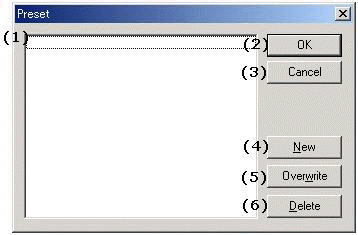
| No. | Button | Description |
| (1) | List box | The preset which ware saved previously are listed. |
| (2) | OK | Reproduces the preset selected on the list box. |
| (3) | Cancel | Closes this dialogue, without doing anything. |
| (4) | New | Saves the current status. |
| (5) | Overwrite | Overwrites the preset selected on the list box by the current status. |
| (6) | Delete | Deletes the preset selected on the list box. |
A keyboard shortcut is a combination of keys that can be pressed to do something that you normally do with the mouse. This topic instructs how to find and use keyboard shortcuts in RA.
For example, as in the figure below, items in the menu bar start with underbars like Window. This means that you can press Alt + W to see the window menu. The buttons on the RA's main window also have shortcuts (Signal Generator, FFT Analyzer, Oscilloscope, and so).
Some of the buttons on the measurement window also have shortcuts. The most useful one might be the Start / Stop key. To start and stop the measurement, just press the S key. In other window, several buttons have shortcuts as well. Check the measurement window and find useful shortcuts.
| Yoshimasa Electronic Inc. |
| TOP | STORE | DSSF3 | RAE | RAD | RAL | MMLIB | Support | Contact Us |