| Japanese | English |
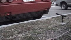
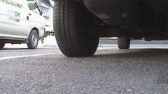
In our first experiment, we placed PC and the microphone at the parking lot to measure the car exhaust and engine sound. However, it was very hard to operate PC in outside. The operation sound of PC had always been recorded. We were very bothered because we had to stop the measurement one by one. Also, when we analyzed data after the measurement, we could not grasp the situation of the measurement. So we had to measure again.
Then, we tried to record sound by a DAT recorder during a measurement, so that we could analyze data later. Once the sound is recorded digitally, it can be measured repeatedly without a loss of information. However, because the measured sounds were very similar in every time, it was hard to discriminate the experimental conditions by only hearing them. We keenly recognized that the picture of the measurement situation should be recorded at the same time.
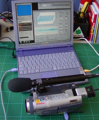
A digital video camera (DV camcorder) that is capable of 16bit, 48kHz sampling can record sound at the same quality as DAT recorder. A digital video can be connected to PC very easily by using the digital interface (e.g. SONY iLINK). So we thought only the digital video camera is enough as the measurement equipment. Compact video camera is very convenient for the outdoor measurement. It is very clear what sound was measured at that time. One important thing to remember is that the built-in microphone of the digital video camera is not good in sound quality. Generally, the external microphone is also necessary for the accurate measurement. This is also same for the DAT recorder. See the following pages for some information about the microphone.
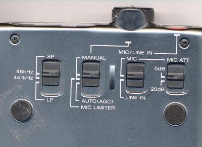
Also, it is important the recording level should be able to be controlled manually. Normally, the digital video camera and the DAT recorder is equipped with a function, called Automatic Gain Control (AGC) to deal with a wide range of input signal levels. AGC assures a fixed predefined output level by automatically compensating input levels. For example, low level signals are boosted and high level signals are attenuated to an average level. This is a convenient function in recording a variety of sound in an appropriate level. But it is sometimes harmful because it has a tendency to introduce audio noise and hiss into the audio signal. For the sound measurement, recording level should be set slightly below the expected maximum sound level to avoid the distortion. The photo below is of DAT recorder.
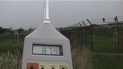
If we want to measure the sound pressure level (SPL) from the recorded sound, there is another important thing to do before starting the recording. It is a calibration of the recorded signal. Without calibration, you can measure only the relative sound level. What is important is to know the actual SPL of the sound recorded on the tape. Sound level meter is used for calibration.
Basic recording and measurement procedure
Record a reference tone before the measurement
After the recording level is adjusted to an appropriate level, record a reference signal (1kHz sine tone of about 10 seconds) to the video tape. At the same time, measure its SPL using a sound level meter. For example, if the measured SPL is 90 dB, the reference signal recorded in the tape can also be defined as 90 dB. This value will be used later when the sound is imported to the computer and measured using the Realtime Analyzer. Note that the recording level should be kept same throughout the actual measurement. If the recording level is changed, the calibrated SPL can't be measured. In that case, the reference tone should be recorded again.
Transfer sound to computer
How to transfer video or sound into the computer is different for each
machine. Suppose that you are ready to replay sound in your computer. In our
experiment, video was transferred to the computer via iLINK connection and
played back by VAIO DVgate-motion.
Calibrate the input level of the Realtime Analyzer
Start Realtime Analyzer and set the input device as WAVE (if the tape is connected to Line-in, the input device should also be Line-in).
Open FFT analyzer > Calibration window, and click the Edit button. When you replay the reference tone recorded on the tape, the Input Level display (dB) will increase. Adjust the scrollbar to the level of the reference tone (e.g. 90dB). Enter the microphone info and click "New" button to save the calibration data. Click OK to go back to the analyzer window. Calibration is now completed.
Confirm the calibration result
Open the Octave band tab. Check that the calibration data saved is selected. Measurement will start by clicking the Start button. Replay the reference tone again. You will see that the SPL of the reference signal will appear as the calibrated level. After that, the calibrated SPL can be measured for the rest of the recordings.
Measure SPL of recorded sound
We are ready to measure SPL of the sound recorded on the tape. Replay the portion of sound to be measured and start the Realtime Analyzer. Changes in SPL in each frequency band can be observed in real-time. Even if we don't calibrate the input level, the relative sound level can be measured correctly. Below is an example of the aircraft noise, reported in Airport Noise Analysis Test 2. SPL data can be exported as a text file by using the data record function. See Measurement data management in Realtime Analyzer.
Sound recording by the Realtime Analyzer
In DSSF3, the running ACF in RA (Real-time Analyzer) and EA (Environmental-noise Analyzer) can be used to record sound and save it as .wav files. In most of our measurement reports, those functions are used. Usually, we record sound in real time and analyze later. It is important to have the original sound in order to check the validity of measurement results. Also, once the sound is saved, analysis can be repeated any number of times.
In the running ACF measurement, sound data and additional information such as the measurement date, sampling rate, signal duration are saved together.
Recorded sound can also be saved as a .wav format. This file can be replayed by Windows Media Player, or can be manipulated by the sound editing software, such as "CoolEdit" (now, it is sold as Adobe Audition). You can edit and postprocess the sound waveform directly. Wave file is read again and it can be saved in the measurement database of DSSF3. It is possible to reproduce sound, and re-analyze with different conditions. Because of the digital processing in the software, the same result is obtained as measuring on real time. Generally, operation takes much time for the high-resolution measurement. So, it is good to set the resolution low in the real-time measurement and reanalyze later. Sound reproduction function can be used to see the real time power spectrum, the octave analysis, and the 3-d display simultaneously. When performing such parallel processing, we recommend you to use the multitasking OS, such as Windows2000 Pro.
Examples of the running ACF measurement from a digital video recording
Measurement of piano music 1 -- Analysis of a wave file, Integral time and 3D displaywave
Even you do not want the running ACF analysis, this function can be used as a sound recorder. Shortly after getting used, you come to be able to perform dynamic analysis of the Running ACF. Many examples are reported in this site.