| TOP | STORE | DSSF3 | MMLIB | Contact Us |
Reference manual for Realtime Analyzer of DSSF3
We are now working for improving the program manual. At the moment, we have added supplementary notes to increase information in the reference manual. We hope these notes help some users, but it might be difficult to read because some descriptions are redundant and vague. At first, read the plain description of the program controls summarized in the table below the screen shots of the program. If you have any questions about the manual, please feel free to contact us.
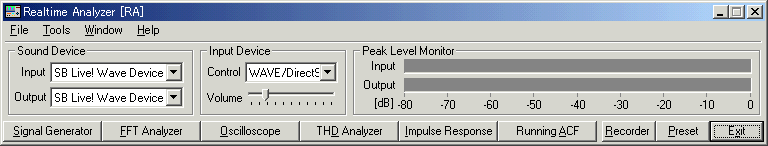
Selection of the input and output device is done in the main window of RA. Adjustment of the input volume is done by the Windows volume control or by the volume control in RA's main window. These two controls are interlinked for ease of use. Measurement functions such as signal generator and FFT analyzer can be accessed from the named buttons in the bottom of the main window.
| Menu | Item | Description |
| File (F) | Exit (X) | Quit the application. |
| Tool (T) | ||
| Settings (S) | Adjust the font size and the window size for each measurement window. -> How to adjust the font size and window size | |
| Window (W) | Signal generator (S) | Open / close the signal generator window. |
| FFT analyzer (F) | Open / close the FFT analyzer window. | |
| Oscilloscope (O) | Open / close the oscilloscope window. | |
| Impulse response (I) | Open / close the impulse response window. | |
| Running ACF (A) | Open / close the running ACF window. | |
| Preset (P) | Open / close the preset window. | |
| THD analyzer (D) | Open / close the THD analyzer window. | |
| Recorder (R) | Open / close the recorder window. | |
| Current time (T) | Open / close the current time window. | |
| Help (H) | Version information (V) | Show the version information. |
| Read me (R) | Open the read me file. | |
| Online manual (M) | Open the online manual (only when connected to the Internet). | |
| Technical support (S) | Open the technical support page (only when connected to the Internet). | |
| Document Q&A (Q) | Open the Q&A page (only when connected to the Internet). | |
| Online update (U) | Execute the online update (only when connected to the Internet, and available only in Version 5.x.x.x.). | |
| License registration (L) | Open the registration dialog. | |
| Buying YmecStore (Y) | Open the purchase page (only when connected to the Internet). |
*Alphabets after the item name (_) show the shortcut keys.
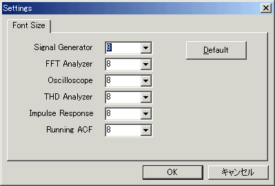
How to adjust the font size and the window size
Select the Tool > Settings from the menu bar. The setting dialog appears as below. Choose the font size for each measurement window and click the OK button. Font size and window size are changed. See the figures below to compare the size. Click the Default button to set them as default values (8 point).
1-2. "Input Device" and "Peak Level Monitor"
| Item | Description |
| Input Device | Selection of an input device. It is same as the Windows volume control. Available input device for the sound card used is displayed (e.g. Microphone, Line-in, CD, WAVE, Mixer). When measuring digital signal, choose WAVE or Mixer (this name depends on your computer or sound driver). |
| Volume | Adjustment of the input signal volume. Normally, the peak level should be below -5 dB for preventing the distortion. |
| Peak Level Monitor | |
| Input | Peak level monitor of an input signal. |
| Output | Peak level monitor of an output signal. This level can be adjusted only by the digital volume in signal generator. When playing wav files (in the Recorder, Running ACF or the Impulse response), peak level of that file is displayed in real time. |
| Sound device | |
| Input | Sound device for input is specified. |
| Output | Sound device for output is specified. |
1-3. Function buttons on the main window of RA
| Buttons | Descriptions |
| Signal Generator | Tone, noise, sweep and pulse is generated as a stereo signal. As for tone, sinusoidal, triangle, square, and saw-tooth wave can be chosen. Each channel can generate different signals with specified frequencies. White, pink, and brown noise can be chosen. Sweep is a tone signal whose frequency is varied continuously. Pulse signal is generated with specified number of time, duration and interval. |
| FFT Analyzer | Two channels spectrum analyzer, 1/1 to 1/24 octave band analyzer, 3D display (TEF or waterfall), correlation meter (auto- and cross-), phase meter, and spectrogram can be chosen. |
| Oscilloscope | Two channels oscilloscope. Auto triggering, level adjustment, X-Y mode (Lissajous pattern). |
| Impulse Response | The impulse response of a room is measured automatically with MLS (Maximum Length Sequence) or TSP (Time Stretched Pulse) methods. Measured impulse response can be saved as wav files. Impulse response files (only wav) measured by the other measurement system can be imported. |
| Running ACF | The running ACF (autocorrelation function) and CCF (cross-correlation function) is measured. It is a time domain sound analysis method. Sound can be recorded up to 30 seconds. Recorded sound can be played and saved as a wav. format. A wav. format sound file can be imported. |
| Preset | Setup of RA can be stored as a "preset." By loading a preset, all settings of RA will be recovered. Each preset is named and comment can be added. This function not only shortens the preparation time before the measurement, but also reduces a mistake. It is highly recommended to use preset for precise measurement. |
| THD Analyzer | Total Harmonic Distortion analyzer. Manual measurement of up to 30th harmonics, level sweep, and frequency sweep measurements are available. |
| Recorder | Sound recorder and player that cooperates with all analyzer functions. |
In the signal generator, several kinds of the test signals (tone, noise, sweep, pulse) are generated. Recently, new functions "Synthesis" and "Scale" have been added. These functions allow easy generation of the complex tone and the musical scale in a various waveforms.
Note
Selection of the output device is a same operation as in Windows. When the sound is output from the loudspeakers, RA outputs the digital signal (WAVE signal) to the Windows sound mixer. Output volume is adjusted by the Windows volume control. To output the sound to external devices (e.g. amplifier), select "line" as the output device in Windows volume control.
Adjustment of output volume is done by Windows volume control. Output volume of the signal is adjusted on the Windows volume control and PC's hard volume. Another important function to control the output volume is "Digital Output" in the signal generator. This is an original function of RA. This volume adjusts the range of the digital signal, to make the signal not to be distorted. It is important to remember that many soundboards' performance becomes poor around their maximum output level.
Selection of the input device is a same operation as in Windows. To measure the sound and other signals by RA, selection of the soundcard and other input device, volume control, and combination of several input devices are controlled in Windows volume control.
Operation of the input microphones is same as in usual sound recording. Usually, "line" is used as the input device. If your PC does not have the line-in terminal, use the microphone input terminal. Alternatively, a soundcard with USB interface is available. Adjustment of the input volume is done by the Windows volume control or by the volume control in RA's main window. These two controls are interlinked for ease of use.
Basic measurement procedure
Input sound can be listened to, be displayed and be measured at the same time. For the measurement of the performance of audio devices, input the test signal (by use of the signal generator) to the device and measure its output by the oscilloscope or the FFT analyzer. Measurement results can be saved as a picture file by using the Windows screen copy function (Alt + PrtScr). Our image database software, MMLIB, is also convenient.
Common items in the Signal Generator
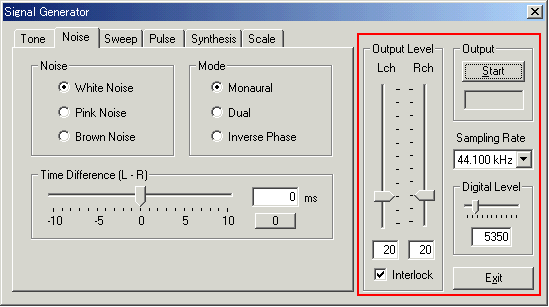
Note: The figure above is the signal generator window (Noise generator is selected). Just below the output "Start" button, elapsed time will be displayed. Sampling rate is now set to 44.1 kHz. There are two volume controls in this window. One is the "Digital Level", that controls the output level of the digital signal to the D/A converter. It is now set to 32767, meaning that the range of the digital signal is between -32767 and +32767 (maximum level in 16 bit resolution). But it is important to remember that most D/A converter causes distortion with such a high output level. Another is the "Output Level", that controls the analog amplifier's output level (after the D/A conversion). In addition, Windows volume control works to adjust the volume of the built in loudspeaker or the line-out. Note that adjusting the signal generator's output level and Windows volume control does not change the level of the digital signal. These volumes only work for the output of the loudspeaker or the line-out. Three volume controls mentioned are connected in series. It is important to adjust them not to cause distortion and to improve the S/N ratio at the same time. For how to do this, see the operation guide in the program manual.
| Name | Description |
| Output | The output of sound signals starts by clicking the [Start]
button. There is a stopwatch function. Time counter starts by clicking on the [Start] button and the time counter is displayed here during the output. The count lasts until the output is finished. |
| Sampling Rate | Number of sampling per second. Hardware is automatically checked and the available sampling rate is displayed. Generally, it is enough to use 44 kHz or 48 kHz. |
| Digital Level | Controls the output level of the digital signal that is fed into the D/A converter. This volume should be reduced if the output signal is distorted. |
| Output Level | Adjustment of the analogue output level after the D/A converter. When the [Interlock] box is checked, left and right channels are outputted as the same level. This control is linked with the Windows' volume control. |
| Exit | Signal Generator program finishes. |
In the tone generator, four kinds of waveforms (sinusoidal, triangle, square, sawtooth) are created. Its frequency is set by entering the numerical values, by moving the slider, or by choosing from presets. Frequency range of the slider bar can be chosen from the menu. Phase difference (degree) between channels can be specified. The phase, or time delay, can be seen in the oscilloscope or the phase meter. Phase can be adjusted to reproduce stereo signals without time delay at the listening position.
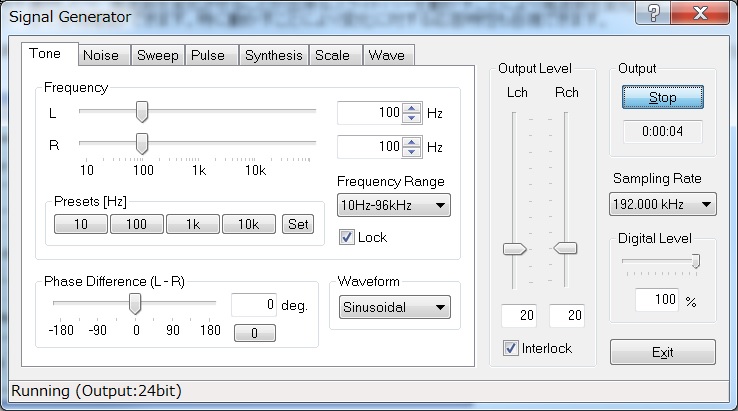
Note: The figure below is the signal generator window during the operation. The elapsed time is displayed as 21 sec. The output level is set separately for L and R channels. Output levels (54 and 43) are expressed in %. This level is set by entering values or by moving the sliders. Frequency is set to 300 Hz in both channels. Frequency is also set by entering values or by moving the sliders. Frequency range of the slider bar can be chosen from the menu. Now the range between 100 and 1kHz is chosen, so the small adjustment is easier than the figure above (10Hz-20kHz is chosen). Also, the preset frequency of "1k" is now changed to "300". This was done by setting the frequency (to 300 Hz), clicking the "Set" button and then "1k" button. Similarly, "10k" is changed to "500".
Waveform of the output tone is sinusoidal and triangular in the above and the below examples. In the above example, phase difference is also changed to -135 deg. Digital level is changed to 29423. All signals created in the signal generator will be compressed between ±29423 to remove the distortion.
Items in Tone generator
| Item | Description |
| Frequency | Specify a frequency by the numerical value or by the slider. When the [Interlock] box is checked, left and right channels are set equal. |
| Waveform | Choose the waveform of output sound from [Sinusoidal], [Triangular], [Square] and [Sawtooth]. Arbitrary waveform stored in the "Wave" tab can also be selected. |
| Presets | Frequency of output signals can be saved as presets. To save the presets, click the "Set" button. Then specify the frequency by the slider or by entering the value. Finally click one of four presets buttons. Once the frequency is saved as a preset, that frequency is shown on the preset button. Default presets are 10, 100, 1k, and 10k Hz. |
| Frequency range | Select the frequency range from the list. Then the range of the slider is changed. |
| Phase difference | Set the phase difference (Left - Right) between two channels in the range between -180 and +180 degree. |
* Four kinds of the waveform
In the noise generator, white noise, pink noise, and brown noise can be generated. Stereo signal can be generated as monaural, dual, and inverse modes. Those difference can be seen by the phase meter.
Time difference between channels can be set between ± 10 ms. Tone generator sets the phase difference between channels in "degree", but noise generator sets the time difference between channels in "ms". This is because the absolute phase depends on the frequency and it cannot be set in the noise signal. In the example shown below, pink noise is generated with the time difference of 0.1 ms.
Items in Noise generator
| Field | Item | Description |
| Noise | White Noise | White noise contains equal energy for all frequency. Its power spectrum is flat. |
| Pink Noise | Pink noise contains equal energy for all octave frequency. Energy decreases for high frequency. Its octave band spectrum is flat. | |
| Brown noise | Power spectrum of the brown noise decreases as the inverse square of its frequency (1 / f2). | |
| Mode | Monaural | Outputs the same signal for left and right channels. |
| Dual | Outputs a different signal for each channel. | |
| Inverse Phase | Outputs an inverse-phased signal for each channel. | |
| Time difference | Specify the time difference between two channels in the range between -10 and +10 ms. | |
Note:
The above signal is displayed as below in the phase meter of the FFT analyzer. In the phase meter, the phase spectrum is displayed in real time.
Sound waveform is not recovered by only the amplitude spectrum. Phase of each frequency component is important. If there is no phase delay, each sinusoidal wave is simply added, but if there is a phase delay, it becomes complicated. If the peaks of two waveforms are synchronized, they are added, but if the peak and the dip are synchronized, they are subtracted. Two sinusoidal waves with the same frequency increases the sound level 6 dB when they are added in-phase, but they become zero when added out-of-phase. The adjustment of time delay is as important as the adjustment of the frequency response (amplitude spectrum).
Signal generator can also generate a sweep signal. Sweep is a tone signal of which frequency is changed continuously between the specified range (From, To) with the specified speed. In the logarithmic sweep, the frequency increases with a fixed rate of octave change per time (octave/sec). This means that every octave contains the same energy. Its long time spectrum is same as the pink noise.
Sweep is a good signal for testing the loudspeaker. Waterfall display with a sweep signal is a very useful measure for the crossover network of the loudspeaker. By changing the sweeping frequency range and its speed, it can be tested in a various way.
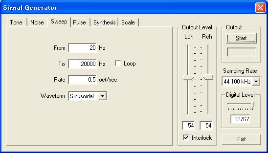
Items in Sweep generator
| Item | Description |
| From To |
The frequency sweep is generated from the frequency inputted in the [From] to the frequency inputted in the [To]. This is the logarithmic sweep, of which the frequency increases with a fixed rate of octave change per time. It means that the energy is constant within octave bands and it decreases at 3dB/oct. |
| Loop | Normally, a sweep signal is outputted only once. If [Loop] is checked, the output is repeated. |
| Rate | Sweep Rate [octave/sec]. |
| Waveform | Select the waveform of output sound. |
Pulse signal is generated with specified length, number of time, interval, and polarity. This is used for the measurement of the impulse response or the polarity of the loudspeaker.
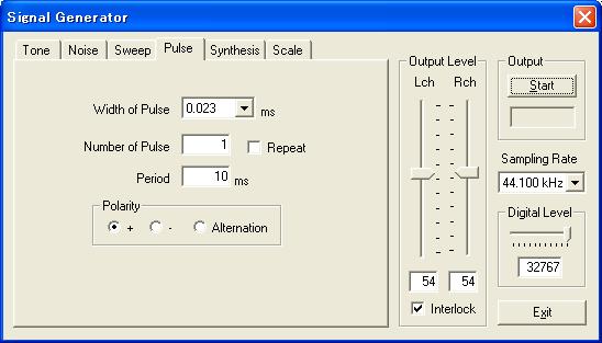
Items in Pulse generator
| Item | Description |
| Width of Pulse | Specify a width of pulse [ms]. |
| Number of Pulse | Specify a number of output pulses. If [Repeat] is checked, number of pulses are repeated until the Stop button is clicked. |
| Period | Specify a period of the pulses [ms]. |
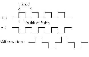
| Polarity | Specify a polarity of pulses.
 |
Note:
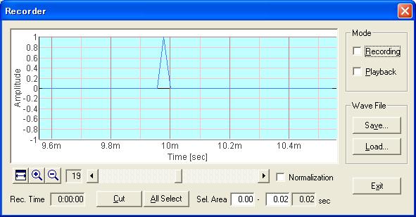
On the pulse generator window, the width of pulse is set to 0.023 ms. Number of pulse is 1 and its period is 10 ms. To check the waveform of this pulse, the recorder is used as below. Open the recorder window and check the "Recording" mode. Then click the start button on the signal generator. Output signal is automatically recorded. The figure below is the result. One pulse is recorded at 10 ms.
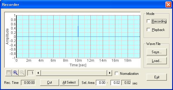
The recorded waveform is zoomed in to x19 in the figure below. In this figure, we can see that the very short pulse with the maximum volume is recorded. If the width of pulse was set to longer values, the waveform becomes square. If the polarity was set to "-", the amplitude becomes minus values.
The recorded sound can be saved as a wav format. A wav file can also be loaded on the recorder, and by using the "Playback" mode, it is automatically measured by the FFT analyzer or the oscilloscope.
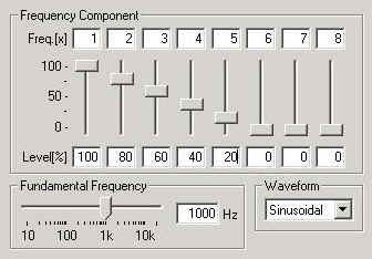
A complex tone can be created easily on the Synthesis window. Set the fundamental frequency and select its waveform, then enter the harmonic number (Freq.[x]) and its relative level (Level[%]).
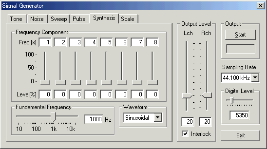
Items in Synthesis
| Item | Description |
| Freq. [x] | Specify the overtones as .x times of the fundamental frequency. |
| Level [%] | Specify the levels of the overtones in %. |
| Fundamental frequency | Specify the fundamental frequency of the signal by the slider or enter the value. |
| Waveform | Select the waveform of output sound. |
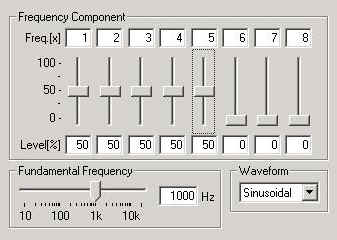
Examples of complex tones
| Left: Signal generator, Right: FFT analyzer | |
| Ex.1: Fundamental frequency is 1000 Hz, overtones are x1, x2, x3, x4, and x5 with levels of 50 %. | |
 |
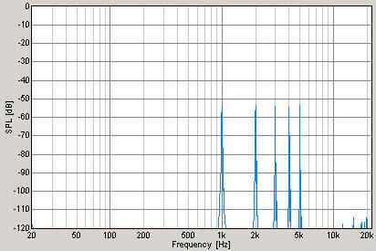 |
| Ex.2: Fundamental frequency is 1000 Hz, overtones are x1-x5, with levels of 100, 80, 60, 40, 20 %. | |
 |
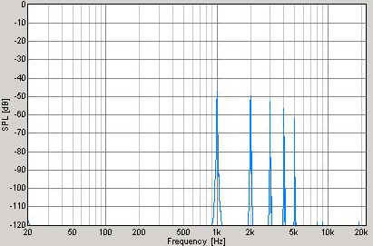 |
Musical scale generator is another new function. Check the "Play Mode" and click the keyboard to play a tone of that note. The frequency can also be specified by selecting the scale and the octave. Selected note is indicated on the keyboard by a green mark.
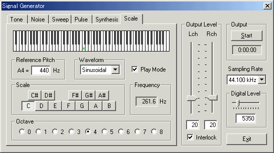
Note:
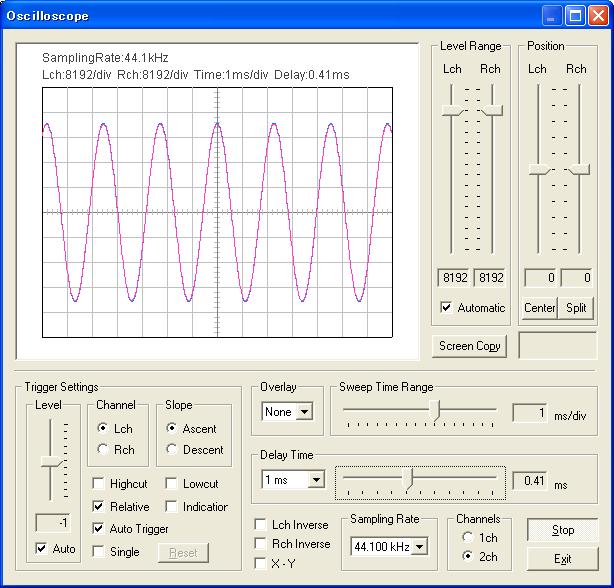
Waveform of the output signal is displayed on the oscilloscope as below.
Items in Scale
| Item | Description |
| Reference Pitch | Enter the frequency of A4. Default value is 440 Hz. |
| Waveform | Select the waveform of output sound. |
| Play Mode | Check here to play sound when clicking on the keyboard. |
| Scale | Specify the scale of note. |
| Frequency | Frequency of the selected scale is shown here. |
| Octave | Specify the octave of note. |
In the newly added Wave tab of the signal generator, arbitrary waveform can be created in the waveform editor and stored up to five waveforms. A signal can be tested by the oscilloscope or the spectrum in real-time, while editing the waveshape. Stored waveforms can be generated in an arbitrary frequency and in a sweep mode.
Items in Wave
| Item | Description |
| Waveform | Select the stored waveform. Selected waveform is displayed above. |
| Edit | Open the waveform editor window. |
| Frequency | Set the frequency of the signal by moving the slider by entering the value. Edited waveform is generated in this frequency. |
Waveform Editor window
Items in the Waveform Editor
| Item | Description |
| Graph area | One period of the waveform is displayed. X axis is a relative time, and Y axis is amplitude. Vertical and horizontal axes can be zoomed up to x512 respectively. |
| Position | Position [X, Y] of the selected vertex is displayed. |
| Edit Mode | Add vertex: Check this and click on the graph to add a new
vertex. Select vertex: Check this and click on the graph to select a vertex. Selected vertex is shown in a red point. Position of the vertex can be changed by dragging on the graph or by entering X, Y positions. |
| Delete vertex | Click this button to delete a selected vertex. |
| All clear | Click this button to delete all vertices. |
| Start | Click this button to start generating the currently edited waveform. Its waveform can be observed by the oscilloscope or the FFT analyzer. |
| Spline curve | Mark this checkbox to create a spline curve that interpolates vertices. |
| OK | Click this button to store the waveform. |
| Cancel | Click this button to do nothing and go back to the signal generator. |
Channel mode (previously, 1ch or 2ch) has been extended to Mono, Stereo,
Left only, Right only, L-R difference. (2005/10/15)
FFT analyzer is a powerful tool for measuring sound in real time. Power spectrum, Octave band analysis, Waterfall display, Correlation meter (auto- and cross-), Phase meter, and Spectrogram can be used.
Note:
Measurement screen can be saved as a picture file by using the Windows screen copy function (Alt + PrtScr). We also recommend the image database software, MMLIB. This software works with all other Windows applications. Attached image of email or Fax is easily stored in the multimedia database.
WAVE file, CD
Signal generator's output can be saved as a wav format in the hard disk or in the CD. Then, these files can be used as test signals instead of the signal generator.
Simultaneous operation
Signal generator, sound recorder, FFT analyzer, and oscilloscope works simultaneously, unless input / output device conflicts. Capability of this operation depends on PC's performance.
Microphone calibration
For the measurement of the absolute sound level, an input level sensitivity can be calibrated. The sound level meter or the acoustic calibrator can be used for the calibration. Microphone's frequency response can also be compensated on the RA's calibration window, if you have the data provided from the manufacturer. This compensation is useful if you are measuring the frequency response of the audio device, such as the amplifier and the loudspeaker.
Use the sound level meter as a microphone
AC-OUT of the sound level meter is the amplified sound itself. It is same as measuring with the microphone and microphone amplifier. RA turns your PC into the sound level meter equipped with the octave band analyzer, the peak hold function, and the TEF (time / energy / frequency) analyzer.
3-1. Common setting items of the FFT analyzer
| Commands or options | Descriptions |
| Input | Measurement starts with the [Start] button. Time counter starts when the Start button is clicked. The elapsed time is displayed here during a measurement. |
| Calibration | Microphone calibration data is managed. ->3-3. Microphone calibration |
| Level | Peak level or total level for L (= left) and R (= right) are displayed in [dB]. By a left-click on the graph, the level and the frequency at the cursor's location is displayed. By a right-click, the cursor on the graph disappears and the total level is displayed. |
| Frequency | Peak frequencies for L (= left) and R (= right) are displayed in [Hz], when the cursor appears on the graph. When the cursor disappears, it is shown as [All]. |
| Resolution | Time resolution and frequency resolution are displayed. F: frequency resolution [Hz]. T: time resolution [ms]. Appendix: more info about time resolution and frequency resolution |
| Split L-R | If this checkbox is marked, screen is split in two and data for two channels are displayed separately. |
| Exit | Finishes the "Realtime Analyzer". |
| Level Range | Set the display range of the sound pressure level (= vertical axis). Automatic and manual setting is available. |
| Freq. Range | Set the display range of the frequency (= horizontal axis). Automatic and manual setting is available. |
| Sampling Rate | Set the sampling rate of A/D conversion. |
| FFT Size | A block size of FFT (Fast Fourier Transform). It can be chosen between 1024 and 65536. Large FFT size causes fine frequency resolution and rough time resolution. Default setting can be used in most cases. |
| Time Window | The time window is used to decrease extra frequencies. Six window functions are available. Default setting can be used in most cases. |
| Freq. Weighting | Select the frequency weighting filter from Flat, A-weighting, B-weighting, and C-weighting. Normally, Flat weighting is recommended. For measuring the noise level, A-weighting is commonly used. |
| Channel Mode | Mono (L+R): Measured in a monaural mode of the soundcard. Stereo: Two channels are measured (left: blue, right: pink) Left only: Only left channel is measured Right only: Only right channel is measured Differ (L-R): Difference of L-R channels is measured [Note] In a monaural mode (Mono), some sound cards input only the left channel, but some cards mixes both channels into one channel. To measure only one channel input, use Left only or Right only mode. |
| Freq. Axis | Setting of the scale of the frequency axis. Logarithm: Rate of the frequency is constant in this scale. Linear: Difference of the frequency is constant in this scale.. |
| Time Resolution | Refresh speed of the real-time display is specified. "1x" (standard), "2x" (double), "4x" (4 times), and "8x" (8 times) can be chosen. |
| Moving Average | When the time is specified (1sec to 10sec, or Infinite), the average value for this period is displayed. |
| Smoothing (T.C.) | Smoothing coefficient is specified as time constant (ms or s). Standard sound level meter settings (fast: 125 ms or slow: 1s) are available. |
| Peak Detection | Peak: A peak location is indicated by the blue crossing (In the case of 2 channels, blue and red). |
| Peak Hold: Peak values are held for some seconds. Auto Reset: peak indication is refreshed with the specified period. Manual Reset: peak indication is refreshed when the "Reset" button is clicked. |
|
| Number of Data | The number of time axes which are displayed in "Waterfall". |
| Direction of Axis | Direction of the time axis in "Waterfall" and "Spectrogram". When [Forward] is selected, the time shifts forward on the screen. When [Backward] is selected, the time shifts backward. |
| Correlation | ACF: Auto-correlation is displayed. CCF: Cross-correlation is displayed. Moving the "Zoom" slider makes it possible to zoom the correlation function to a suitable scale on time-axis. |
| Maximize button Close button |
|
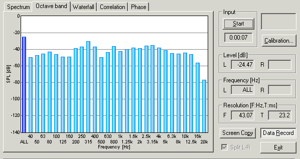
| Octave band | Bandwidth of the octave band analysis is selected from 1/1 to 1/24. |
| Screen Copy | Click to capture the snapshot of the measurement screen. You can record any number of measurement screens during a measurement. It is convenient for comparison and printing of measurement results. |
| Data Rec. | Click to open the data logging window (only available in the octave band analyzer). Time series data of the octave band level with a specified interval can be saved as a .CSV format. ->3-4. Data record |
| Display | Description |
| Spectrum | Measures the power spectrum of the input signal. Sound level is displayed as a function of frequency. |
| Octave band | Octave band analysis is performed. Energy at each octave band is displayed in real time. 1/1, 1/3, 1/6, 1/12, and 1/24 octave is available. |
| Waterfall | Time-energy-frequency analysis is performed. Results are displayed in the 3D graph. |
| Correlation | Auto- and Cross-correlation functions are measured. |
| Phase | Phase difference between channels is displayed as a function of frequency. |
| Spectrogram | Energy at a given time and frequency is displayed as a color map in the 2D diagram. |
For the measurement of the sound pressure level (SPL), an input level sensitivity can be calibrated. The sound level meter or the acoustic calibrator can be used for the calibration. Microphone's frequency response can also be compensated, if you have the data provided from the manufacturer. This compensation is useful if you are measuring the frequency response of the audio device, such as the amplifier and the loudspeaker.
This is a convenient function even though you don't need to calibrate SPL. Once the input level is adjusted and saved in the calibration window, input volume is re-adjusted automatically when the calibration data is selected.
Read Operation guide 3. Microphone setting for a step by step instruction of microphone calibration.
Items in the Calibration dialog
| Items | Description |
| Calibration Data list | Calibration data already stored in the database is displayed. |
| OK | Applies the selected calibration data. |
| Release | Releases the already applied calibration data. |
| Cancel | Closes the dialog without doing anything. |
| Edit | Opens the edit window for the calibration data. |
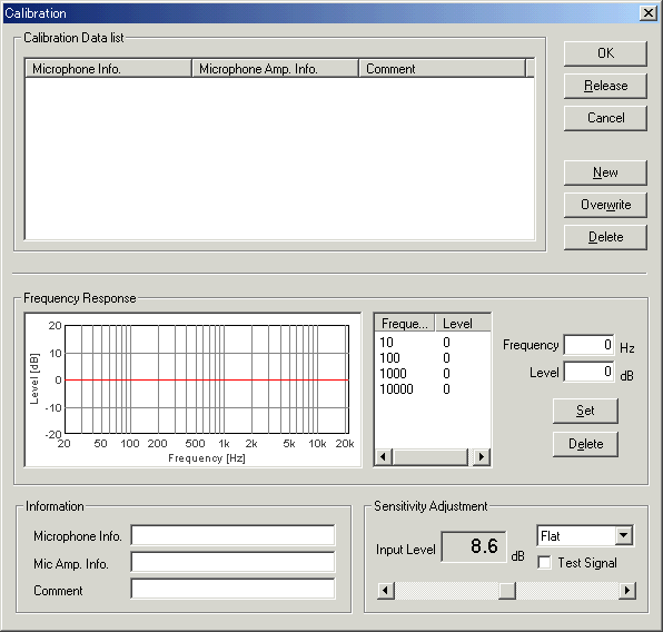
Items in the Calibration dialog, edit window
| Items | Description |
| Calibration Data list | Calibration data already stored in the database is displayed. |
| OK | Applies the selected calibration data. |
| Release | Releases the already applied calibration data. |
| Cancel | Closes the dialog without doing anything. |
| New | Saves the new calibration data. |
| Overwrite | Makes a change to the already stored calibration data. |
| Delete | Deletes the selected calibration data. |
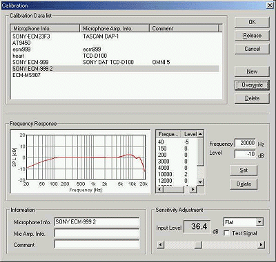
| Frequency response | Frequency response data is edited for compensation. The frequency response curve is created by entering [Frequency] and [Level] values. Only four frequencies of 10, 100, 1000, and 10000 are appeared in the list, but the new frequency values can be added by entering the number in the Frequency box and clicking the [Set] button. |
| Information | Microphone Info., Mic Amp. Info. (optional), and Comment (optional) can be saved with the calibration data. |
| Sensitivity Adjustment | Input level is indicated in dB. Frequency weighting can be selected from Flat, A-, B-, C-weighting. The input level can be adjusted by moving the scrollbar. Test signal (1kHz tone) can be generated. Note that the sensitivity adjustment for measuring the absolute sound pressure level must be done with the sound level meter or the acoustic calibrator. |
Note: Supplement explanation of microphone calibration
If you are using two or more microphones, or doing measurements in different settings, you can store the calibration data for each setting. The calibration data can be used as a preset for the input device settings. Once you save the calibration data, input volume is re-adjusted automatically when that calibration data is selected.
It is important that a wide dynamic range and a high S/N ratio are obtained. So the calibration should be done by increasing the input level as much as possible with the expected sound level in the actual measurement. If necessary, several different calibration data can be used for different input sound level.
In the following example, the frequency response curve of Sony ECM-999 is edited, before the measurement of the loudspeaker's frequency response. This microphone covers a wide frequency range and a wide dynamic range. By compensating the frequency curve, more accurate measurement would be possible.
But note that the microphone compensation is recommended only for the frequency response measurement by using pink noise or white noise. For measuring transient sounds, we recommend to use the high quality microphone without compensation. It is because the amplitude spectrum (i.e. frequency response) can be compensated, but the phase spectrum (i.e. transient response) can not be compensated. Ideally, the microphone should have a flat frequency response and transient response to capture sound accurately, but generally it is not. Most microphones are adjusted so that they have balanced frequency response and transient response. If only the frequency response is compensated, its transient response is distorted. It is no problem for measuring the stationary sound such as pink noise and white noise, but it causes problems for measuring the transient sound (music, speech, etc.).
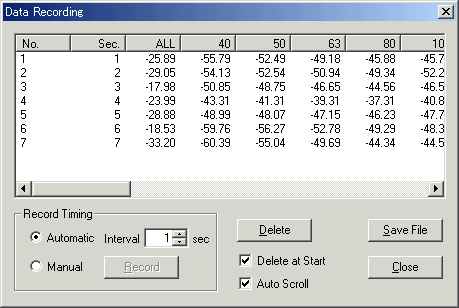
Data record function is available for the octave band analyzer. Click the "Data Record" button to open the Data Recording dialog. Measured sound pressure levels in all-pass and each octave band frequency can be recorded. This data can be saved as a CSV format, which can be manipulated by other applications like Microsoft Excel.
Note:
On the Data Recording window, record timing can be selected from automatic and manual. In the automatic mode, data is recorded in every interval. Minimum recording interval is 1 second. In the manual mode, data is recorded when the Record button is clicked.
For example, select the Automatic for record timing and start the measurement in the FFT analyzer. Then the octave band level is recorded automatically. Recorded data can be save as a CSV format, which is manipulated by other applications like Microsoft Excel. Time history of the sound pressure level, basic statistics (max, min, average, percentile), equivalent sound pressure level (Leq), noise criteria (NC) values can be easily calculated.
Items in the Data Recording dialog
| Items | Description |
| Data list | Measurement data is displayed. |
| Record Timing | Automatic: Measured data is recorded
automatically with the specified interval. Manual: Measured data is recorded when the "Record" button is clicked. |
| Delete | Deletes all data. |
| Delete at Start | Recorded data is deleted when the measurement is started. |
| Auto Scroll | Latest data is already displayed by scrolling the data list. |
| Save File | Saves the recorded data as .csv or .txt format. |
| Close | Closes the Data Recording dialog. |
NEW: Channel mode (previously, 1ch or 2ch) has
been extended to Mono, Stereo, Left only, Right only, L-R difference.
(2005/10/15)
The oscilloscope shows the waveform of the input signal in real time. No difficult settings can be ignored first. By just clicking the Start button, input signal is triggered and the level range is adjusted automatically. The waveform is displayed in the proper positions.
The waveform of the input signal is observed. Vertical axis is amplitude and
horizontal axis is time. When "X-Y" check box is marked, horizontal axis is left
channel's amplitude and vertical axis is right channel's amplitude. The mark ![]() on the left of window indicates the point of trigger start level.
on the left of window indicates the point of trigger start level.
Note:
When the input and the output signals are to be compared by the 2ch mode, it is important to remember that it is not possible to select different input devices (for example, line-in and wave) at the same time. It is a limitation of Windows' sound control. So, the signals to be measured should be fed into the separate channels of the same input device.
For example, let's consider the situation to measure the audio amplifier's output. We want to input the sinusoidal wave to the amplifier, measure the output of the amplifier, and compare it with the input waveform to know how much the signal is changed. In this case, one signal is the signal generator's output (this is the input to the amplifier) and another is the amplifier's output. To compare these signals, connect the Right channel of the soundcard's output directly to the Right channel input of the sound card (for measuring the signal generator's output), connect the Left channel output to the amplifier (for feeding the signal generator's output to the amplifier), and connect the amplifier's output to the Left channel input of the sound card (for measuring the amplifier's output).
Then, start the signal generator and the oscilloscope. You can see two waveforms (one is the input signal, and another is the output of the amplifier) on the oscilloscope screen at the same time. It can be easily observed whether the signal is correctly amplified, whether the signal is distorted or not. By changing two inputs of the soundcard, any signals can be compared similarly.
Check the following application notes for how to use the oscilloscope.
http://www.ymec.com/hp/signal2/oscillo.htm
http://www.ymec.com/hp/signal2/oscillo2.htm
Snapshot of the measurement screen can be easily taken by the Screen Copy button. Automatic over sampling is applied to the signal to display the smoothed waveform especially for the short sweep time range.
4-1. Items of the Oscilloscope
| Item | Description | |
| Level Range | Decides a value of one grid of the vertical axis in the oscilloscope display. For example, when the Level Range is set to 1, one grid becomes 1. When the Level Range is set to 32768, one grid becomes 32768. When the [Automatic] checkbox is marked, this value is set automatically so that the signal is displayed in an appropriate range. | |
| Position | Vertical position of the waveform is adjusted by the slider
for each channel. If [Center] button is clicked, the waveform is arranged at the middle of the window. If [Split] button is clicked, two waveforms are arranged vertically. |
|
| Overlay | Automatic over sampling is applied to the signal to display the smoothed waveform especially for the short sweep time range. | |
| Sweep Time Range | Time range of one grid on the horizontal axis [ms]. For displaying a low frequency signal, Sweep Time Range should be set to large. For example, to see one cycle of 1 Hz tone, Sweep Time Range has to be larger than 100ms/div. However, the calculation load becomes high at such a condition. It might be difficult to display a signal smoothly if you use a slow PC. | |
| Delay Time | An interval from the input to the display [ms]. Select the time range from 1ms, 10ms, 100ms, and 1000ms in a popup menu. Then, adjust the delay time (= It is shown in the box) with the slider. For example, when you select "1ms" from a popup menu, The scale of the slider becomes 0-1 ms. |
|
| Trigger Settings | Trigger settings are adjusted here. | |
| Level | Trigger level is set up. This is the starting point of a waveform. If the [Auto] checkbox is marked, trigger level is adjusted automatically. | |
| Channel | Select the channel which becomes the object of trigger settings. | |
| Slope | The timing of trigger. - Ascent: When a waveform gets over the trigger level in upward direction, the trigger is pulled. (A waveform starts upward.) - Descent: When a waveform gets over the trigger level downward, the trigger is pulled. (A waveform starts downward.) |
|
| Highcut | High frequency noise is cut. | |
| Lowcut | Low frequency noise is cut. | |
| Relative | If this checkbox is marked, it is indicated relatively. Without a check, an absolute position is shown. | |
| Indication | The starting level of the trigger is indicated with " |
|
| Auto Trigger | If you check here, the waveform will be displayed even when it has no trigger for a certain period of time. | |
| Single | Snapshot of the waveform is created when the [Reset] button is clicked. | |
| Reset | Display is reset with this button, when the [Single] checkbox is marked. | |
| Lch Inverse | Inverts a waveform of left channel up and down. | |
| Rch Inverse | Inverts a waveform of right channel up and down. | |
| X-Y | Plots the left channel as a vertical axis and the right channel as a horizontal axis. This plot is called Lissajous pattern. It is shown with green lines. | |
| Sampling Rate | Sampling rate of the A/D conversion. | |
| Channels | Mono (L+R): Measured in a monaural mode of the soundcard. Stereo: Two channels are measured (left: blue, right: pink) Left only: Only left channel is measured Right only: Only right channel is measured Differ (L-R): Difference of L-R channels is measured [Note] In a monaural mode (Mono), some sound cards input only the left channel, but some cards mixes both channels into one channel. To measure only one channel input, use Left only or Right only mode. |
|
| Start (Stop) | Starts (and stops) an oscilloscope. | |
| Exit | Closes "Oscilloscope". | |
| Screen Copy | Click to capture the measurement screen. | |
Note: Supplementary information of the oscilloscope
The oscilloscope is generally used in checking an operation of electronic circuits. Voltage variations in a short time, or its oscillating waveforms are measured in real time. RA's oscilloscope not only measure the voltage waveform, but also waveforms of various signals through the input devices.
Input devices as below can be used by the oscilloscope.
| Device | Description |
| WAVE | Sound signal generated inside the PC, such as Windows Media Player or RA's signal generator, can be measured. |
| SW synthesizer(MIDI) | Output signal of the SW synthesizer can be measured. |
| CD player | Signal in the CD (test signal or music) can be measured. |
| mic | Signal from the built-in microphones or devices connected to the microphone port can be measured. |
| telephony | Signal from the internal modem can be measured. |
| PCBeep | Phase difference between two channels can be measured. |
The unit of the oscilloscope display is the amplitude of the digitized signal. Its maximum is +-32768 at the time of 16bit sampling. To measure the voltage, it is required to calibrate the input level using the voltmeter. Once the input voltage of the soundcard is calibrated, you can measure the voltage by the oscilloscope. Calibration can be done by feeding a stationary signal (e.g. sine tone) to the soundcard and by measuring its AC voltage.
The software does not have a maximum input voltage limit. Input signal to the oscilloscope is always scaled to the maximum level of the soundcard. Rather, the maximum input voltage is limited by the soundcard (usually it is around 1.0-1.5V). But even if the signal level exceeds the maximum voltage of the soundcard, it can be measured by using attenuator.
THD analyzer measures the Total Harmonic Distortion of the system. THD is a measure to evaluate the linearity of the system, and it is defined as the ratio of the geometric mean of the harmonic components (v1, v2, v3, v4, v5, ... v30) and the fundamental component (v1) when the sinusoidal wave is inputted to the system. Usually it is expressed in dB or %.
In the THD analyzer, three different measurements are available: a) manual measurement, in which the distortion is measured for the specific frequency and the output level, b) frequency sweep measurement, in which the measurement frequency is changed automatically, and c) level sweep measurement, in which the output level is changed automatically.
THD analyzer can measure the distortion of the amplifier very effectively. For example, connect the soundcard's output to the amplifier, and connect the amplifier's output to the soundcard's input. You don't need to connect the soundcard's output and input directly. THD analyzer compares the input and the output signals automatically and gives the result (distortion). Measurement result can be saved as a screen picture. MMLIB can be used to manage the image file.
5-1. Common items of THD Analyzer
| Item | Description |
| Measurement | Measurement starts with the [Start] button. Time counter starts when the Start button is clicked and the elapsed time is displayed here during the measurement. The time count lasts until the output is finished. |
| Sampling Rate | This item sets a sampling rate of A/D conversion. |
| Channels | 1ch: One channel (light blue) 2ch: Two channels (light blue and red) |
| Max Harmonics | This item sets the maximum harmonics that can be measured. Higher order enables correct measurement, but the CPU load also becomes high. |
| Guard Time | This item sets a time interval between the output of a measurement signal and the distortion measurement. |
| Scale | This item sets the unit of the distortion (% or dB) and the range of the graph (max and min). |
In the manual measurement, distortion is measured for the specified frequency and the output level. The total harmonics distortion and distortion for each harmonics are displayed.
Items of manual measurement
| Item | Description |
| Measurement Frequency | This item sets the frequency to be measured. Move the slider or enter the value. |
| Measurement Level | This item sets the output level. The maximum level of the system is shown as 0 dB. |
| Setting | Check the Averaging box for displaying the averaged results during the measurement. |
| THD | THD (total harmonic distortion) that is currently measured is displayed. |
Back to common items of THD analyzer
5-3. Frequency sweep measurement
In the frequency sweep measurement, the measurement frequency is changed automatically. Results are plotted for each frequency during the measurement.
Items of frequency sweep measurement
| Item | Description |
| Measurement Frequency | Enter the Start frequency, the End frequency, and the number of points to be measured. |
| Measurement Level | This item sets the output level. The maximum level of the system is shown as 0 dB. |
| Setting | Check the Interpolation box for smoothing the distortion graph. Spline interpolation is used. |
| THD | Distortion that is currently measured is displayed. |
Back to common items of THD analyzer
In the level sweep measurement, the output level is changed automatically. Results are plotted for each level during the measurement.
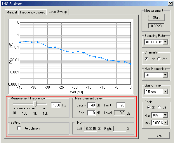
Items of level sweep measurement
| Item | Description |
| Measurement Frequency | This item sets the measurement frequency. |
| Measurement Level | Enter the Start level, the End level, and the number of points to be measured. |
| Setting | Check the Interpolation box for smoothing the distortion graph. Spline interpolation is used. |
| THD | Distortion that is currently measured is displayed. |
Back to common items of THD analyzer
In RA, the impulse response is measured by the simultaneous input and output of the MLS (or TSP) signal. Sampling rate, measurement time, and measurement channel (monaural or stereo) can be specified. Measured impulse response can be saved as a wav format or a text format. Output signal and input signal themselves can also be saved. Measurement data is managed in the common database in RA and SA.
From the measured impulse response, the important room acoustics parameters
are easily analyzed by SA. Sound level, initial time delay gap between the
direct and the reflected sound, reverberation time, and IACC are calculated for
each 1/1 or 1/3 octave band. The impulse response is also used for the
auralization (virtual acoustic reality) and the variety of sound effects, by
using the well established convolution techniques.
Compensation of the loudspeaker and the microphone's response (frequency response and dynamic response) is possible by using the "inverse filter" function. It can be set at the time of measurement. Compensation of the frequency response of the microphone is also available.
Measurement data at many positions in a concert hall are easily managed by
use of RA and SA. At the time of measurement by RA, the measurement conditions
are recorded automatically in the database. Sound level is calculated as a
relative level within a data folder, by specifying one data (or the maximum
level) as a reference level.
RA is equipped with the measurement supporting functions for beginners. In the "Auto Retry" mode, measurement is repeated twice and the accuracy of the measurement is checked by comparing with the test measurement result. By using this function, measurement is repeated until the correct data is obtained. This is a very important function to make a measurement reliable.
See Impulse response guide for the step by step instruction.
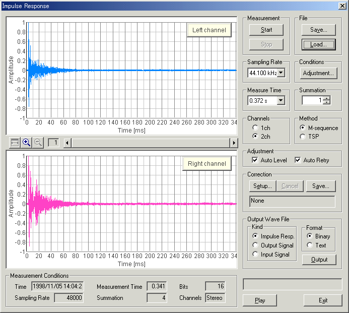
6-1. Items on the Impulse response window
| Field | Description |
| Measurement | The measurement starts with [Start] button. Though the measurement finishes automatically, you can stop it with [Stop] button. |
| File | [Save...] button: Saves the data measured here. See:
6-2. Save measurement data [Load...] button: Loads the data stored previously. See: 6-3. Load measurement data |
| Sampling Rate | Available sampling rates of the sound card used are displayed. |
| Conditions | [Adjustment...] button: Input / output level, microphones position, measurement time are adjusted automatically. See: 6-4. Adjustment |
| Measure Time | The time duration for measuring the impulse response. It is automatically adjusted. |
| Summation | The number of times that the measured impulse responses are added and averaged out. If this number becomes larger, S/N ratio is improved. But the time duration becomes longer. |
| Channels | Choose stereo (= 2 channels) or monaural (= 1 channel). |
| Method | The MLS method and the TSP method can be used in the impulse response
measurement. It can be used only by choosing one of the MLS and the TSP. TSP is a signal in which the energy of an impulse is distributed on the time axis. In the TSP method, an impulse response is calculated by generating TSP signal, acquiring the response and returning the dispersed energy. |
| Auto level | It is adjusted so that an output level can become the most suitable.
(The output signal is amplified within the range that the input doesn't
become saturated, and S/N ratio is improved.) If you turn "Auto Level" off. You can adjust the sound volume (output level) using Windows sound volume control. |
| Auto Retry | Measurement will be repeated until distortion-free data can be obtained. You can release it at your option by switching on/off. |
| Correction | Unwanted response of the measurement system including microphone and
loudspeaker is removed. [Setup...] button: Sets the Inverse filter. [Cancel] button: Cancels the Inverse filter. [Save...] button: Saves new Inverse filter. |
| Output Wave File | The data are saved in wave file format and text file format. |
| Play | Clicking on this enables to listen to the impulse response sound. |
| Exit | "Impulse Response" program is finished. |
| These buttons adjust the range of indication of impulse response. | |
| Measurement Conditions | Various conditions of the measurement are shown. (Time, Measurement Time, Bits, Sampling Rate, Summation, Channels) |
By clicking [Save...] button on the "Impulse Response" window, the following "Save Measurement Data" window appears. The measured data will be stored in a folder.
When you measure the impulse response at many positions in a concert hall, save data in the same folder. Sound level will be calculated as a relative level within a data folder, by specifying one data (or the maximum level) as a reference level.
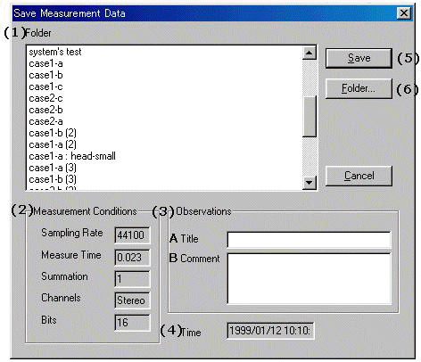
| No. | Field | Description |
| (1) | Folder | The folders, in which the measured data are stored, are listed. |
| (2) | Measurement Conditions | The measurement conditions of measured data are indicated. |
| (3) | Observations | Input the information about the data to save. |
| (3)-A | Title | Input data's name. |
| (3)-B | Comment | You can make optional comments upon the data. |
| (4) | Time | The time and date when data were measured. |
| (5) | Save | Saving is carried out. |
| (6) | Folder... | The folders in which the data are stored are managed. You can create new folder, alter the information such as folder's name, and delete a folder. |
| 1. | Select the folder to save data; |
| From [Folder] list box , select the folder into which you want to save the measured data. If you want to save in a new folder, click [Folder...] button and create a new folder there. | |
| 2. | Input data's name; |
| Input the name of measured data into [Title] text box. And input the other information into [Comment] text box if necessary. | |
| 3. | Save the data; |
| Carry out with [Save] button. If you want to cancel, click [Cancel] button. |
<Folder Management>
Clicking [Folder...] button on "Save Measurement Data" window, the following
"Folder Management" window appears.
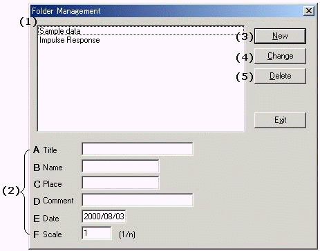
| No. | Button and Field | Description |
| (1) | - | The folders, in which the measured data are stored, are listed. |
| (2) | - | Information about the folder. |
| (2)-A | Title | Folder's name. |
| (2)-B | Name | The person who carried out the measurement. (Optional) |
| (2)-C | Place | The place where the measurement were done. (Optional) |
| (2)-D | Comment | Optional information. (Optional) |
| (2)-E | Data | The date when the folder was created. It is set automatically. |
| (2)-F | Scale | In the case of experiment with a model, its scale is inputted. For example, you measured the impulse response for 1/10 scale model, you should input "10" in the box. |
| (3) | New | Creates a new folder, which has the information you have inputted to (2). The new folder appears in the list box. |
| (4) | Change | Changes the information about the folder which is selected in the list
box. Select the folder in the list box, and the information about this folder are displayed in (2). Alter the information in (2) and then click this button. |
| (5) | Delete | Deletes the folder which is selected in the list box. |
Back to Items on the Impulse response window
Clicking [Load...] button on "Impulse Response" window, the following dialog
appears. Select the impulse response data you want to load. Wav files of 8, 16,
32 bit can be loaded.
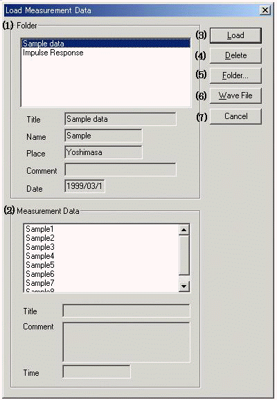
| No. | Field and button | Description |
| (1) | Folder | The folders, in which the measured data are stored, are listed. Here, select the folder which includes the data you want to load. The information (Title, Name, Place, Comment, and Date) about selected folder are shown below the list box. |
| (2) | Measurement Data | The data which are included in the folder selected in [Folder]
list box (1) are listed. Here, select the data you want to load. The information (Title, Comment, and Time) about selected data are shown below the list box. |
| (3) | Load | Loads the data selected in [Measurement Data] list box (2). |
| (4) | Delete | Deletes the data selected in [Measurement Data] list box (2). |
| (5) | Folder... | Opens [Folder Measurement] dialog. |
| (6) | Wave File | Loads wave file. |
| (7) | Import | Imports database of DSSF3/RAE/RAD. |
| (8) | Cancel | Closes this dialog without doing anything. |
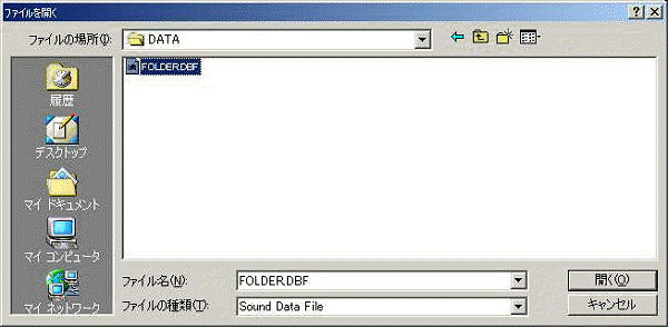
Database of the impulse response measurement can be imported from DSSF3/RAE/RAD on other PC.
Open the shared drive on your LAN.
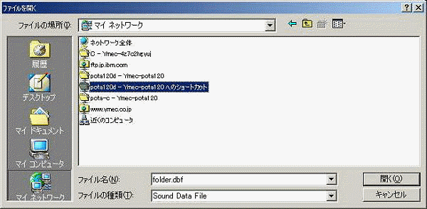
Open database of DSSF3.
Back to Items on the Impulse response window
The following adjustment is not necessary if you can measure correctly. If you find difficulties, follow the instructions below.
RA has a function to check the measurement conditions. If it were not good, it can be adjusted automatically. Click the "Adjustment" button on the Impulse response window to open the Adjustment dialog as a figure below. Items to be checked are "Input Output Level", "Mic. Position", and "Measuring Time". They are displayed OK when the settings are correct.
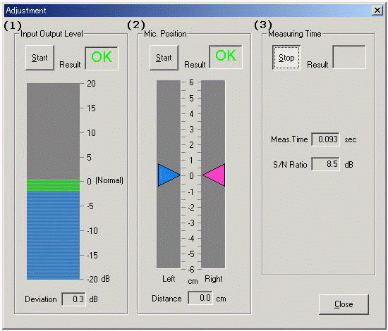
| No. | Field | Description |
| (1) | Input Output Level | By clicking [Start] button, a signal sound is outputted. Then,
adjust the volume of amplifier to the level marked with [Normal]. A result is indicated, "OK" or "NG". |
| (2) | Mic. Position | The difference between the distances from the sound source to left and right microphones is indicated in Distance text box. Adjust this value to "0". |
| (3) | Measuring Time | According to the size of reverberation in the sound field, the most
suitable time for measuring is set. When the measurement time is shorter in comparison with the reverberation time, the measurement is not carried out exactly. And, when the measurement time is too long, it takes long time to measure and calculate. |
Back to Items on the Impulse response window
6-5. Correction (inverse filter setting)
[Save] the inverse filter
In this window, the inverse filter is created from the measured impulse response. Only the initial part of the response should be selected because the response of the measurement system is included in this part.
| No. | Fields | Description |
| (1) | Impulse Response | Measured impulse response is shown. The yellow area represents a
filtering range. Adjust the boundary of the yellow area, so as to include the part which is thought of as the impulse response of the measurement system within the yellow area. Drag left and right borderlines when the mouse cursor shape changes to "<-| |->" over borderline. |
| (2) | Filtering | Characteristics (Level, Phase) of the inverse filter corresponding to
the impulse response which is cut out from (1) are indicated. Red curve is characteristic of sound pressure level, and green curve is the phase characteristic. |
| (3) | Title | Input the name for the present inverse filter. |
| (4) | Comment | Input the comment on the present inverse filter. |
| (5) | Maximum Level | Sets the SPL limit for correction of the inverse filter. |
| (6) | Phase Correction | When this box is checked, both SPL and phase are corrected. If not, only SPL is corrected. Ordinarily, it should be checked. |
| (7) | Save | Saves the inverse filter. |
| (8) | Exit | Closes this dialog. |
[Setup] the inverse filter
To set the filter, click the "Setup" button and select the filter. Then start
the measurement. The impulse response of a room excluding the response of the
measurement system can be measured.
| No. | Field | Description |
| (1) | (List box) | The inverse filters which have been stored are listed. |
| (2) | Impulse Response | Measured impulse response is shown. The yellow area represents a
filtering range. Adjust the boundary of the yellow area, so as to include the part which is thought of as the impulse response of the measurement system within the yellow area. Drag left and right borderlines when the mouse cursor shape changes to "<-| |->" over borderline. |
| (3) | Filtering | Characteristics (Level, Phase) of the inverse filter corresponding to
the impulse response which is cut out from (2) are indicated. Red curve is characteristic of sound pressure level, and green curve is the phase characteristic. |
| (4) | Title | The name of the present inverse filter. |
| (5) | Comment | The comment on the present inverse filter. |
| (6) | Maximum Level | Sets the SPL limit for correction of the inverse filter. |
| (7) | Phase Correction | When this box is checked, both SPL and phase are corrected. If not, only SPL is corrected. Ordinarily, it should be checked. |
| (8) | OK | Applies the selected inverse filter to the measurement. |
| (9) | Cancel | Closes this dialog without doing anything. |
| (10) | Overwrite | Saves the altered inverse filter. |
| (11) | Delete | Deletes the selected inverse filter. |
Back to Items on the Impulse response window
Conventional sound level meter measures sound level by two time constants, fast: 125 ms and slow: 1.0 s. Octave band analyzer measures the averaged sound levels in each frequency band. These methods are effective for the almost stationary sound, but are not helpful for measuring the time varying sound.
Instead, the running ACF measurement analyzes sound in the time domain by setting two parameters, the integration time and the running step. These parameters decide the averaging time and the calculation interval, respectively. In this way, temporally fluctuating sound is accurately measured. For example, averaged sound level of 0.5 s is calculated in every 0.2 s. Of course, those parameters can be set freely (between 0.001 s and 10 s) according to the target sound. The measured running ACF is displayed as a 3D graph.
Measured ACF data is saved in the measurement database, and analyzed by SA in
detail with any condition. The acoustical parameters can be calculated by the
time resolution up to 1 ms. Subjective attributes of sound, such as loudness,
pitch, pitch strength, reverberation components, and the spatial properties of
sound source, such as location, width of a source, diffuseness, are analyzed.
Analysis results are stored with its conditions, so the comparison of results is
quite easy.
Furthermore, SA has a powerful graphic function that displays the analysis
results in an intelligible way. In this analysis result display, graphs and
tables for each acoustic parameter are easily treated. For example, clicking the
mark in the graph opens the data at that point. The analysis graphs of the ACF
parameters can be zoomed in/out with a suitable time resolution for the precise
display. Graphs are saved as image files, and tables are saved as a text format.
Such original and powerful functions make analysis of huge amount of data very
easily.
High analysis capability and user-friendly interface are the great features of RA and SA's running ACF measurement. This covers a wide range of application, such as the sound quality analysis of noise, diagnosis of motor and fan, medical diagnosis of auscultation sound, or the analysis of voice quality.
See running ACF guide for the step by step instruction.
7-1. Items on the Running ACF window
| Items | Descriptions | |
| Graph (Upper) | The graph of the Running ACF is displayed. The vertical axis is the autocorrelation, the horizontal axis is the time, and the depth is the running step. | |
| Measurement | The measurement starts with [Start] button. Although the measurement stops automatically if the time you have set passes by, it is possible to stop it with [Stop] button. | |
| File | [Save...] button is used for saving the measured data in a file
(database) See:
7-2. Save measurement data
[Load...] button is used for loading the stored data. See: 7-3. Load measurement data |
|
| Measurement Settings |
Sampling Rate | A sampling rate of A/D conversion. (44.1 or 48 kHz is recommended) |
| Time | Set the time for measuring. | |
| Channels | Choose the number of channel used for measurement, 1 channel (monaural) or 2 channels (stereo). | |
| Display Settings |
Integration Time | Set the Integration Time of ACF between 0.001 and 10 s. |
| Running Step | Set the Running Step (calculation interval) between 0.001 and 10 s. | |
| Time Range | Set the maximum value of the horizontal axis (t) in the graph. | |
| Freq. Weighting | Select the frequency weighting filter. | |
| Number of Data | Set the number of the data on the time axis (= The depth of graph) | |
| Direction | Set the direction of the time axis of the graph. Forward: The time shifts forward. Backward: The time shifts backward. |
|
| Vertical Axis | Set the scale of the vertical axis (Autocorrelation value). Linear: Autocorrelation is indicated in linear scale between -1 and 1. If [Abs.] box is checked, absolute value of Autocorrelation is indicated between 0 and 1. Log: Autocorrelation is indicated in logarithm (decibel) scale. Its range is from 0 dB to the value inputted to the right text box. |
|
| Channel | In the case of stereo measurement, left channel's data is displayed by checking "L ch" radio button, and right channel's data is displayed by checking "R ch" radio button. (Left channel's data is displayed in light blue, and right channel's one is pink.) In the case of monaural measurement, only left channel is displayed. | |
| Redraw | When the setting is changed, clicking on this button displays new data. | |
| Input Wave | The waveform of the input signal is displayed. | |
| Normalization | The input data is normalized between -1 and 1. | |
| Edit | Unnecessary part can be removed from the measured data. [Sel. Area] text boxes: Input the start and the end of the part you want to select. The selected area is painted with light blue. Or, this light blue area is changeable by dragging its left and right borderlines when the mouse cursor shape changes to "<-||->" over borderline. [Cut] button: Cuts off the part except light blue area. [All Sel.] button: Selects the whole area. (The whole area become light blue.) [Replay] button: Outputs the selected part (light blue area) from the speaker. During playback, a green line indicates where is replayed. |
|
| Measurement Conditions | The measurement conditions (Time, Sampling Rate, Measurement Time) are shown. | |
| Exit | Finishes "Running ACF" program. | |
7-2. Save Measurement Data
Clicking [Save...] button on "Running ACF" window, the following "Save
Measurement Data" window appears.
The measured data will be stored in a folder.
| No. | Field | Description |
| (1) | Folder | The folders, in which the measured data are stored, are listed. |
| (2) | Measurement Conditions | The measurement conditions of measured data are indicated. |
| (3) | Observations | Input the information about the data to save. |
| (3)-A | Title | Input data's name. |
| (3)-B | Comment | You can make optional comments upon the data. |
| (4) | Time | The time and date when data were measured. |
| (5) | Save | Saving is carried out |
| (6) | Folder... | The folders in which the data are stored are managed. You can create new folder, alter the information such as folder's name, and delete a folder. ( -> Explained in the following section.) |
| (7) | Wave file | Saves as Wave file. |
| 1. | Select the folder to save data; |
| From [Folder] list box , select the folder into which you want to save the measured data. If you want to save in a new folder, click [Folder...] button and create a new folder there. | |
| 2. | Input data's name; |
| Input the name of measured data into [Title] text box. And input the other information into [Comment] text box if necessary. | |
| 3. | Save the data; |
| Carry out with [Save] button. If you want to cancel, click [Cancel] button. |
<Folder Management>
Clicking [Folder...] button on "Save Measurement Data" window, the following
"Folder Management" window appears.
| No. | Field and button | Description |
| (1) | - | The folders, in which the measured data are stored, are listed. |
| (2) | - | Information about the folder. |
| (2)-A | Title | Folder's name |
| (2)-B | Name | The person who carried out the measurement. (Optional) |
| (2)-C | Place | The place where the measurement were done. (Optional) |
| (2)-D | Comment | Optional information. (Optional) |
| (2)-E | Date | The date when the folder was created. It is set automatically. |
| (2)-F | Scale | In the case of experiment with a model, its scale is inputted. |
| (3) | New | Creates a new folder, which has the information you have inputted to (2). The new folder appears in the list box . |
| (4) | Change | Changes the information about the folder which is selected in the list
box. Select the folder in the list box, and the information about this folder are displayed in (2). Alter the information in (2) and then click this [Change] button. |
| (5) | Delete | Deletes the folder which is selected in the list box. |
Back to Items on the Running ACF window
7-3. Load Measurement Data
Clicking [Load...] button on "Running ACF" window, the following dialog appears.
Select the ACF data you want to load, here.
| No. | Field | Description |
| (1) | Folder | The folders, in which the measured data are stored, are listed. Here, select the folder which includes the data you want to load. The information (Title, Name, Place, Comment, and Date) about selected folder are shown below the list box. |
| (2) | Measurement Data | The data which are included in the folder selected in [Folder]
list box are listed. Here, select the data you want to load. The information (Title, Comment, and Time) about selected data are shown below the list box. |
| (3) | Load | Loads the data selected in [Measurement Data] list box. |
| (4) | Delete | Deletes the data selected in [Measurement Data] list box. |
| (5) | Folder... | Opens [Folder Management] dialog. |
| (6) | Wave file | Opens Wave file. |
| (7) | Import | Imports database of DSSF3/RAE/RAD. |
| (8) | Cancel | Closes this dialog without doing anything. |
Back to Items on the Running ACF window
8. Sound recorder
Sound recorder window has been newly added to RA. Recording of sound up to about
10 minutes is possible. Playback of the recorded sound can be measured by the
FFT analyzer (e.g. Spectrum, octave analysis, oscilloscope, ACF/CCF measurement)
at the same time.
How to use sound recorder
To start recording, check the Recording box on the Recorder window. Then, start one of the Signal Generator, the FFT Analyzer, or the Oscilloscope. When the FFT Analyzer or the Oscilloscope is started, the input signal is recorded. When the Signal Generator is started, the generated signal is recorded. To stop recording, click the Stop button of the window that was started.
Right click on the recorded waveform and drug the mouse to change the selection. Selected region is displayed in blue. Click the Cut button to cut out the selected range. Click the Save button to Save the recorded signal as the wave file (.wav format).
Click the Load button to Load the wave file. Loaded wave file can be played and analyzed as the recorded sound. Sampling rate of the analyzer is automatically set to that of the wave file.
| Item | Description |
| Mode | Select the operation mode of the recorder.
Recording: Check this box and start the analyzer to start recording. |
| Rec. Priority | When the signal input and output are performed at the same
time (e.g. at the time of measuring the speaker response by using the pink
noise), selected source is recorded.
Input: Input signal is recorded. |
| Wave File | Save: Click this button to save the recorded signal as a
.wav format. Load: Click this button to load the already saved .wav files. |
| Normalization | The recorded signal is normalized between -1 and 1. Note that the normalization is done only for the display. Actual signal amplitude is not changed when the signal is analyzed or saved in a file. |
| These buttons adjust the display range of the recorded signal. | |
| Rec. Time | Elapsed recording time is displayed. |
| Cut | Cut the selected waveform area. Unselected area is abandoned. |
| All Select | Select the full time range of the waveform. |
| Sel. Area | Selected area of the waveform is indicated. |
This function is very useful for shortening the preparation time and for reducing the mistakes in the measurement. If you are using the software in a group, settings for each user can be managed separately.
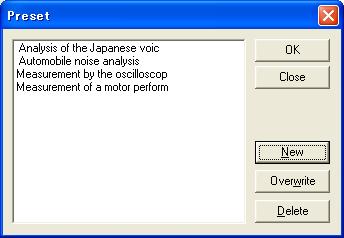
| Button | Description |
| List box | The preset which ware saved previously are listed. |
| OK | Reproduces the preset selected on the list box. |
| Cancel | Closes this dialogue, without doing anything. |
| New | Saves the current status. |
| Overwrite | Overwrites the preset selected on the list box by the current status. |
| Delete | Deletes the preset selected on the list box. |
A keyboard shortcut is a combination of keys that can be pressed to do something that you normally do with the mouse. This topic instructs how to find and use keyboard shortcuts in RA.
For example, as in the figure below, items in the menu bar start with underbars like Window. This means that you can press Alt + W to see the window menu. The buttons on the RA's main window also have shortcuts (Signal Generator, FFT Analyzer, Oscilloscope, and so).
Some of the buttons on the measurement window also have shortcuts. The most useful one might be the Start / Stop key. To start and stop the measurement, just press the S key. In other window, several buttons have shortcuts as well. Check the measurement window and find useful shortcuts.
| Y Store. |
| TOP | STORE | DSSF3 | MMLIB | Contact Us |
If you have questions or comments about this
page,
feel free to contact us by email ymec@ymec.com
or by online
inquiry form.